Mathematical Preliminaries
In this chapter, we briefly review the basic mathematical concepts that are required to understand the materials of this book.
Metric Space
A metric space (\mathcal{X},d) is a set \mathcal{X} together with a metric d on the set. Here, a metric is a function that defines a concept of distance between any two members of the set, which is formally defined as follows.
Definition 1 A metric on a set \mathcal{X} is a function called the distance d : \mathcal{X}\times \mathcal{X}\mapsto {\mathbb R}_+, where {\mathbb R}_+ is the set of non-negative real numbers. For all x, y, z \in \mathcal{X}, this function is required to satisfy the following conditions:
d(x, y) \geq 0 (non-negativity).
d(x, y) = 0 if and only if x = y.
d(x, y) = d(y, x) (symmetry).
d(x, z) \leq d(x, y) + d(y, z) (triangle inequality).
Before going further it is worth seeing that the axioms are satisfied by more than the familiar distance, and that they do exclude things.
Example 1 The following are metric spaces.
The Euclidean metric d({\boldsymbol{x}},{\boldsymbol{y}})=\|{\boldsymbol{x}}-{\boldsymbol{y}}\|_2 on {\mathbb R}^n.
The discrete metric on any set, d(x,y)=1 if x\neq y and 0 otherwise. Every subset is open under it, so it is a useful source of counterexamples.
The supremum metric on C[a,b], the continuous functions on [a,b], d(f,g)=\sup_{t\in[a,b]}|f(t)-g(t)|. Convergence in this metric is uniform convergence.
The metric induced by any norm on a vector space, d({\boldsymbol{x}},{\boldsymbol{y}})=\|{\boldsymbol{x}}-{\boldsymbol{y}}\|, of which the l_p metrics of the l_p norms are the family we use most.
By contrast, the squared Euclidean distance d({\boldsymbol{x}},{\boldsymbol{y}})=\|{\boldsymbol{x}}-{\boldsymbol{y}}\|_2^2 is not a metric: with x=0, y=1, z=2 on the real line it gives d(x,z)=4 while d(x,y)+d(y,z)=2, so the triangle inequality fails. It is nonetheless a perfectly good objective function, which is why the distinction matters — being a useful measure of discrepancy and being a metric are different things.
A metric on a space induces topological properties like open and closed sets, which lead to the study of more abstract topological spaces. Specifically, about any point x in a metric space \mathcal{X}, we define the open ball of radius r>0 about x as the set
\begin{aligned} B_r(x)=\{y\in \mathcal{X}:d(x,y)<r\}. \end{aligned}
Using this, we have the formal definition of openness and closedness of a set.
Definition 2 A subset U\subset \mathcal{X} is called open if for every x \in U there exists an r > 0 such that B_r(x) is contained in U. The complement of an open set is called closed.
A sequence (x_{n}) in a metric space \mathcal{X} is said to converge to the limit x\in \mathcal{X} if and only if for every \varepsilon >0, there exists a natural number N such that d(x_{n},x)<\varepsilon for all n>N. A subset \mathcal{S} of the metric space \mathcal{X} is closed if and only if every sequence in \mathcal{S} that converges to a limit in \mathcal{X} has its limit in \mathcal{S}. In addition, a sequence of elements (x_{n}) is a Cauchy sequence if and only if (iff) for every \varepsilon> 0, there is some N \geq 1 such that
d(x_n, x_m) < \varepsilon,\quad \forall\quad m,n \geq N.
We are now ready to define the important concepts in metric spaces.
Definition 3 A metric space \mathcal{X} is said to be complete if every Cauchy sequence converges to a limit; or if d(x_n, x_m) \rightarrow 0 as both n and m independently go to infinity, then there is some y\in \mathcal{X} with d(x_n, y) \rightarrow 0.
Completeness is a property of the space, not of the metric alone. The rationals {\mathbb Q} with d(x,y)=|x-y| are not complete: the sequence 1, 1.4, 1.41, 1.414,\ldots is Cauchy in {\mathbb Q} but its limit \sqrt2 is not a rational number. The same sequence in {\mathbb R} converges. This is the sense in which {\mathbb R} completes {\mathbb Q}, and it is why the iterative algorithms mentioned above are stated over {\mathbb R}^n rather than over the numbers a computer can actually represent.
We turn now to maps between metric spaces. Continuity is defined first in the general form, and the Lipschitz condition afterwards as a stronger requirement.
Definition 4 Let (\mathcal{X},d_{\mathcal{X}}) and (\mathcal{Y},d_{\mathcal{Y}}) be metric spaces. A function f:\mathcal{X}\mapsto \mathcal{Y} is continuous at x_0\in \mathcal{X} if for every \varepsilon>0 there exists \delta>0 such that
d_{\mathcal{X}}(x,x_0)<\delta \quad \Longrightarrow \quad d_{\mathcal{Y}}(f(x),f(x_0))<\varepsilon . \tag{1}
It is continuous if it is continuous at every point, and uniformly continuous if the same \delta works at every point, i.e. if for every \varepsilon>0 there is a \delta>0 such that d_{\mathcal{Y}}(f(x),f(y))<\varepsilon whenever d_{\mathcal{X}}(x,y)<\delta.
Two equivalent formulations are worth recording, because each is the convenient one in a different argument. First, f is continuous if and only if the preimage f^{-1}(V) of every open V\subset \mathcal{Y} is open in \mathcal{X} — the formulation that survives when the metric is dropped and only the topology is kept. Second, f is continuous at x_0 if and only if f(x_n)\to f(x_0) for every sequence x_n\to x_0, which is the one used to pass a limit through a function.
Definition 5 Given two metric spaces (\mathcal{X}, d_{\mathcal{X}}) and (\mathcal{Y}, d_{\mathcal{Y}}), where d_{\mathcal{X}} denotes the metric on the set \mathcal{X} and d_{\mathcal{Y}} is the metric on set \mathcal{Y}, a function f:\mathcal{X}\mapsto \mathcal{Y} is called Lipschitz continuous if there exists a real constant K\geq 0 such that, for all x_1,x_2\in \mathcal{X},
\begin{aligned} d_{\mathcal{Y}}(f(x_{1}),f(x_{2}))\leq K d_{\mathcal{X}}(x_{1},x_{2}). \end{aligned}
Here, the constant K is often called the Lipschitz constant, and a function f with the Lipschitz constant K is called K-Lipschitz function.
The three conditions stand in a strict hierarchy,
\text{Lipschitz} \;\Longrightarrow\; \text{uniformly continuous} \;\Longrightarrow\; \text{continuous}, \tag{2}
and neither implication reverses. Taking \delta=\varepsilon/K in Equation 1 proves the first, and the second is immediate from the definitions. For the failures: f(x)=\sqrt{x} on [0,1] is uniformly continuous but not Lipschitz, since its slope is unbounded near 0; and f(x)=x^2 on {\mathbb R} is continuous but not uniformly continuous, since the \delta that works near the origin fails far from it. The distinction is not academic here — a Lipschitz gradient is exactly the hypothesis under which gradient descent with a fixed step size is guaranteed to descend.
Vector Space
A vector space \mathcal{V} is a set that is closed under finite vector addition and scalar multiplication. In machine learning applications, the scalars are usually members of real or complex values, in which case \mathcal{V} is called a vector space over real numbers, or complex numbers.
Stated in full, a vector space over a field {\mathbb F} (for us {\mathbb R} or {\mathbb C}) is a set \mathcal{V} with an addition and a scalar multiplication satisfying, for all {\boldsymbol{u}},{\boldsymbol{v}},{\boldsymbol{w}}\in \mathcal{V} and \alpha,\beta\in{\mathbb F}:
{\boldsymbol{u}}+{\boldsymbol{v}}={\boldsymbol{v}}+{\boldsymbol{u}} and ({\boldsymbol{u}}+{\boldsymbol{v}})+{\boldsymbol{w}}={\boldsymbol{u}}+({\boldsymbol{v}}+{\boldsymbol{w}});
there is a zero vector \mathbf{0} with {\boldsymbol{u}}+\mathbf{0}={\boldsymbol{u}}, and each {\boldsymbol{u}} has an inverse -{\boldsymbol{u}} with {\boldsymbol{u}}+(-{\boldsymbol{u}})=\mathbf{0};
\alpha(\beta {\boldsymbol{u}})=(\alpha\beta){\boldsymbol{u}} and 1{\boldsymbol{u}}={\boldsymbol{u}};
\alpha({\boldsymbol{u}}+{\boldsymbol{v}})=\alpha {\boldsymbol{u}}+\alpha {\boldsymbol{v}} and (\alpha+\beta){\boldsymbol{u}}=\alpha {\boldsymbol{u}}+\beta {\boldsymbol{u}}.
A subspace of \mathcal{V} is a subset that is itself a vector space under the same operations. Verifying the eight axioms again is unnecessary: a non-empty \mathcal{W}\subset \mathcal{V} is a subspace precisely when it is closed under linear combination, that is when \alpha {\boldsymbol{u}}+\beta {\boldsymbol{v}}\in \mathcal{W} for all {\boldsymbol{u}},{\boldsymbol{v}}\in \mathcal{W} and all scalars \alpha,\beta. Every subspace contains \mathbf{0}, which is the quickest way to rule one out.
For example, the Euclidean n-space {\mathbb R}^n is called a real vector space, and {\mathbb C}^n is called a complex vector space. In the n-dimensional Euclidean space {\mathbb R}^n, every element is represented by a list of n real numbers, addition is component-wise, and scalar multiplication is multiplication on each term separately. More specifically, we define a column n-real-valued vector {\boldsymbol{x}} to be an array of n real numbers, denoted by
{\boldsymbol{x}}= \begin{bmatrix} x_1 \\ x_2 \\ \vdots \\ x_n \end{bmatrix} = \begin{bmatrix}x_1 & x_2 & \cdots & x_n \end{bmatrix}^\top \in {\mathbb R}^n,
where the superscript ^\top denotes the adjoint. Note that for a real vector, the adjoint is just a transpose. Then, the sum of the two vectors {\boldsymbol{x}} and {\boldsymbol{y}}, denoted by {\boldsymbol{x}}+{\boldsymbol{y}}, is defined by
{\boldsymbol{x}}+{\boldsymbol{y}}= \begin{bmatrix}x_1 +y_1 & x_2 +y_2 & \cdots & x_n+ y_n \end{bmatrix}^\top.
Similarly, the scalar multiplication with a scalar \alpha\in {\mathbb R} is defined by
\alpha {\boldsymbol{x}}= \begin{bmatrix}\alpha x_1 & \alpha x_2 & \cdots & \alpha x_n \end{bmatrix}^\top.
In addition, we formally define the inner product and the norm in a vector space as follows.
Definition 6 Let \mathcal{V} be a vector space over {\mathbb R}. A function \langle\cdot,\cdot\rangle_{\mathcal{V}}:\mathcal{V}\times\mathcal{V}\mapsto {\mathbb R} is an inner product on \mathcal{V} if:
Linear: \langle \alpha_1 {\boldsymbol{f}}_1+\alpha_2 {\boldsymbol{f}}_2, {\boldsymbol{g}}\rangle_{\mathcal{V}}= \alpha_1 \langle {\boldsymbol{f}}_1, {\boldsymbol{g}}\rangle_{\mathcal{V}}+ \alpha_2 \langle {\boldsymbol{f}}_2, {\boldsymbol{g}}\rangle_{\mathcal{V}} for all \alpha_1,\alpha_2\in {\mathbb R} and {\boldsymbol{f}}_1,{\boldsymbol{f}}_2,{\boldsymbol{g}}\in \mathcal{V}.
Symmetric: \langle {\boldsymbol{f}}, {\boldsymbol{g}}\rangle_{\mathcal{V}}= \langle {\boldsymbol{g}}, {\boldsymbol{f}}\rangle_{\mathcal{V}}.
\langle {\boldsymbol{f}}, {\boldsymbol{f}}\rangle_{\mathcal{V}}\geq 0 and \langle {\boldsymbol{f}}, {\boldsymbol{f}}\rangle_{\mathcal{V}}= 0 if and only if {\boldsymbol{f}}=\mathbf{0}.
If the underlying vector space \mathcal{V} is obvious, we usually represent the inner product without the subscript \mathcal{V}, i.e. \langle {\boldsymbol{f}},{\boldsymbol{g}}\rangle. For example, the inner product of the two vectors {\boldsymbol{f}},{\boldsymbol{g}}\in {\mathbb R}^n is defined as
\langle {\boldsymbol{f}}, {\boldsymbol{g}}\rangle = \sum_{i=1}^n f_i g_i = {\boldsymbol{f}}^\top{\boldsymbol{g}}.
Two nonzero vectors {\boldsymbol{x}},{\boldsymbol{y}} are called orthogonal when
\langle {\boldsymbol{x}}, {\boldsymbol{y}}\rangle = 0,
which we denote as {\boldsymbol{x}}\perp {\boldsymbol{y}}. A vector {\boldsymbol{x}} is orthogonal to a subset \mathcal{S}\subset \mathcal{V}, denoted by {\boldsymbol{x}}\perp \mathcal{S}, if it is orthogonal to every element of \mathcal{S}. The orthogonal complement of \mathcal{S}, denoted by \mathcal{S}^\perp, consists of all vectors in \mathcal{V} that are orthogonal to every vector in \mathcal{S}, i.e.
\mathcal{S}^\perp = \{{\boldsymbol{x}}\in \mathcal{V}: \langle {\boldsymbol{v}},{\boldsymbol{x}}\rangle = 0, ~\forall {\boldsymbol{v}}\in \mathcal{S}\}.
Definition 7 A norm \|\cdot\| is a real-valued function defined on the vector space that has the following properties:
\|{\boldsymbol{x}}\|\geq 0, and \|{\boldsymbol{x}}\|=0 if and only if {\boldsymbol{x}}=\mathbf{0}.
\|\alpha {\boldsymbol{x}}\|=|\alpha |\|{\boldsymbol{x}}\| for any scalar \alpha.
Triangular inequality: \|{\boldsymbol{x}}+{\boldsymbol{y}}\|\leq \|{\boldsymbol{x}}\|+\|{\boldsymbol{y}}\| for any vectors {\boldsymbol{x}} and {\boldsymbol{y}}.
The lp Norms
The family we use throughout is the l_p norms, written \|\cdot\|_p. For {\boldsymbol{x}}\in{\mathbb R}^n and p\geq 1,
\|{\boldsymbol{x}}\|_p = \left( \sum_{i=1}^n |x_i|^p \right)^{1/p} , \tag{3}
with the limiting case \|{\boldsymbol{x}}\|_\infty = \lim_{p\to\infty}\|{\boldsymbol{x}}\|_p = \max_i |x_i|. The cases p=1, p=2 and p=\infty account for nearly every norm in this book: \|\cdot\|_2 is the induced norm of the Euclidean inner product, \|\cdot\|_1 is the sparsity-promoting surrogate of the discussion of convexity, and \|\cdot\|_\infty is the dual norm of \|\cdot\|_1, as Table 3 records.
The first two norm axioms are immediate from Equation 3. The third is Minkowski’s inequality, \|{\boldsymbol{x}}+{\boldsymbol{y}}\|_p \leq \|{\boldsymbol{x}}\|_p+\|{\boldsymbol{y}}\|_p for p\geq 1, which is where the restriction on p enters.
It is worth seeing that the restriction is real rather than a technicality. Define \|{\boldsymbol{x}}\|_p by Equation 3 for some 0<p<1 — say p=1/2 — and take
{\boldsymbol{x}}=\begin{bmatrix}1\\0\end{bmatrix},\qquad {\boldsymbol{y}}=\begin{bmatrix}0\\1\end{bmatrix}.
Then \|{\boldsymbol{x}}\|_{1/2}=\|{\boldsymbol{y}}\|_{1/2}=1, while
\|{\boldsymbol{x}}+{\boldsymbol{y}}\|_{1/2} = \left(1^{1/2}+1^{1/2}\right)^{2} = 4 > 2 = \|{\boldsymbol{x}}\|_{1/2}+\|{\boldsymbol{y}}\|_{1/2},
so the triangle inequality fails and \|\cdot\|_{1/2} is not a norm. The geometric statement of the same fact is that the set \{{\boldsymbol{x}}: \|{\boldsymbol{x}}\|_p\leq 1\} is convex for p\geq1 and non-convex for p<1, its faces bending in towards the origin. Such \|\cdot\|_p are called quasi-norms, and they satisfy the triangle inequality only up to a constant.
The non-convexity is exactly why they are used. The count of non-zero entries, written \|{\boldsymbol{x}}\|_0, is the quantity one actually wants to minimise in a sparse recovery problem, and minimising it is combinatorial. The quasi-norms with p<1 approximate \|\cdot\|_0 better than \|\cdot\|_1 does — at the price of the convexity that makes \|\cdot\|_1 tractable. That trade is the subject of a large literature, and the discussion of convexity explains what is lost when convexity goes.
From the inner product, we can obtain the so-called induced norm:
\|{\boldsymbol{x}}\|=\sqrt{\langle {\boldsymbol{x}},{\boldsymbol{x}}\rangle}.
Similarly, the definition of the metric in the metric space section informs us that a norm in a vector space \mathcal{V} induces a metric, i.e.
\begin{aligned} d({\boldsymbol{x}},{\boldsymbol{y}}) = \|{\boldsymbol{x}}-{\boldsymbol{y}}\|,\quad {\boldsymbol{x}},{\boldsymbol{y}}\in \mathcal{V}. \end{aligned}
The norm and inner product in a vector space have special relations. For example, for any two vectors {\boldsymbol{x}},{\boldsymbol{y}}\in \mathcal{V}, the following Cauchy–Schwarz inequality always holds:
\begin{aligned} |\langle {\boldsymbol{x}}, {\boldsymbol{y}}\rangle| \leq \|{\boldsymbol{x}}\|\|{\boldsymbol{y}}\|. \end{aligned} \tag{4}
The proof is short enough to give, and the argument — minimise a quadratic that is non-negative by construction — recurs throughout the book.
Proof. If {\boldsymbol{y}}=\mathbf{0} both sides vanish, so assume {\boldsymbol{y}}\neq \mathbf{0} and take the real case. For every t\in{\mathbb R},
0 \leq \|{\boldsymbol{x}}-t{\boldsymbol{y}}\|^2 = \|{\boldsymbol{x}}\|^2 - 2t\langle {\boldsymbol{x}},{\boldsymbol{y}}\rangle + t^2\|{\boldsymbol{y}}\|^2 .
The right-hand side is a quadratic in t that is never negative, so its discriminant cannot be positive: 4\langle {\boldsymbol{x}},{\boldsymbol{y}}\rangle^2 - 4\|{\boldsymbol{x}}\|^2\|{\boldsymbol{y}}\|^2 \leq 0, which is Equation 4. Equivalently, substituting the minimiser t^\star = \langle {\boldsymbol{x}},{\boldsymbol{y}}\rangle/\|{\boldsymbol{y}}\|^2 gives 0 \leq \|{\boldsymbol{x}}\|^2 - \langle {\boldsymbol{x}},{\boldsymbol{y}}\rangle^2/\|{\boldsymbol{y}}\|^2. For a complex inner product the same argument runs with t chosen to align the phase of \langle {\boldsymbol{x}},{\boldsymbol{y}}\rangle. This concludes the proof.
Equality holds if and only if \|{\boldsymbol{x}}-t^\star{\boldsymbol{y}}\|=0, that is if and only if {\boldsymbol{x}} and {\boldsymbol{y}} are linearly dependent. One consequence is that the induced norm really is a norm: expanding \|{\boldsymbol{x}}+{\boldsymbol{y}}\|^2=\|{\boldsymbol{x}}\|^2+2\langle {\boldsymbol{x}},{\boldsymbol{y}}\rangle+\|{\boldsymbol{y}}\|^2 and bounding the middle term by Equation 4 gives \|{\boldsymbol{x}}+{\boldsymbol{y}}\|^2 \leq (\|{\boldsymbol{x}}\|+\|{\boldsymbol{y}}\|)^2, which is the triangle inequality.
Banach and Hilbert Space
An inner product space is defined as a vector space that is equipped with an inner product. A normed space is a vector space on which a norm is defined. An inner product space is always a normed space since we can define a norm as \|{\boldsymbol{f}}\|=\sqrt{\langle {\boldsymbol{f}},{\boldsymbol{f}}\rangle}, which is often called the induced norm. Among the various forms of the normed space, one of the most useful normed spaces is the Banach space.
Definition 8 The Banach space is a complete normed space.
Here, the “completeness” is especially important from the optimization perspective, since most optimization algorithms are implemented in an iterative manner so that the final solution of the iterative method should belong to the underlying space \mathcal{H}. Recall that the convergence property is a property of a metric space. Therefore, the Banach space can be regarded as a vector space equipped with desirable properties of a metric space. Similarly, we can define the Hilbert space.
Definition 9 The Hilbert space is a complete inner product space.
We can easily see that the Hilbert space is also a Banach space thanks to the induced norm. The inclusion relationship between vector spaces, normed spaces, inner product spaces, Banach spaces and Hilbert spaces is illustrated in Figure 1.
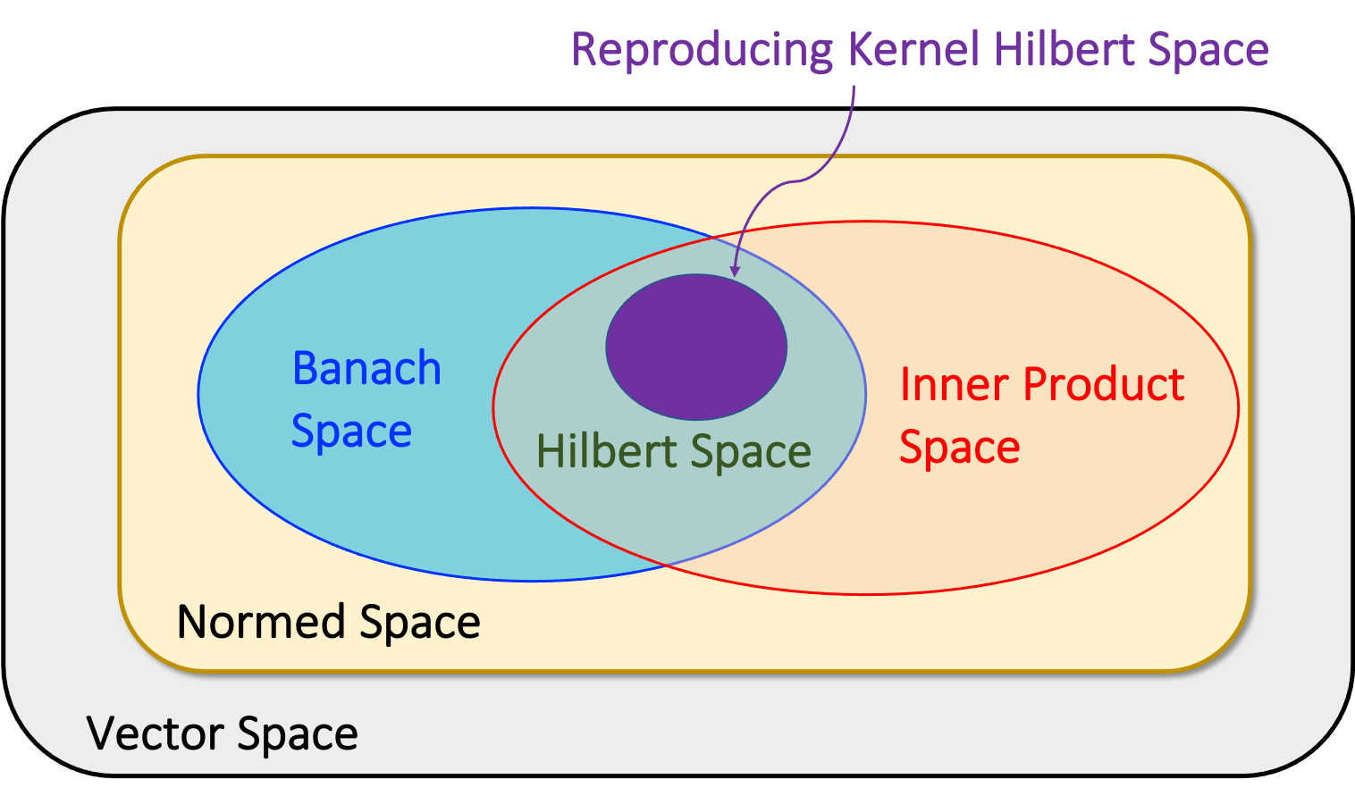
As shown in Figure 1, the Hilbert space has many nice mathematical structures such as inner product, norm, completeness, etc., so it is widely used in the machine learning literature. The following are well-known examples of Hilbert spaces:
l^2(\mathbb{Z}): a function space composed of square summable discrete-time signals, i.e.
l^2(\mathbb{Z})= \left\{ {\boldsymbol{x}}=\{x_l\}_{l=-\infty}^\infty ~\left|\right.~ \sum_{l=-\infty}^\infty |x_l|^2 <\infty\right\}.
Here, the inner product is defined as
\begin{aligned} \langle {\boldsymbol{x}}, {\boldsymbol{y}}\rangle_{\mathcal{H}}=\sum_{l=-\infty}^\infty x_l\overline{y_l}, \quad \forall {\boldsymbol{x}},{\boldsymbol{y}}\in \mathcal{H}. \end{aligned} \tag{5}
L^2({\mathbb R}): a function space composed of square integrable continuous-time signals, i.e.
L^2({\mathbb R})= \left\{ x(t) ~\left|\right.~ \int_{-\infty}^\infty |x(t)|^2 dt <\infty\right\}.
Here, the inner product is defined as
\begin{aligned} \langle x, y \rangle_{\mathcal{H}}=\int x(t)\overline{y(t)} dt. \end{aligned} \tag{6}
Among the various forms of the Hilbert space, the reproducing kernel Hilbert space (RKHS) is of particular interest in the classical machine learning literature. Here, the readers are reminded that the RKHS is only a subset of the Hilbert space as shown in Figure 1, i.e. the Hilbert space is more general than the RKHS.
What distinguishes an RKHS is that pointwise evaluation is well behaved. In a general function space, two functions can be close in norm yet differ wildly at a given point — in L^2({\mathbb R}) the value f(x) at a single x is not even defined, since changing f on a set of measure zero changes nothing.
Definition 10 A Hilbert space \mathcal{H} of functions f:\mathcal{X}\mapsto {\mathbb R} is a reproducing kernel Hilbert space if for every x\in\mathcal{X} the evaluation functional \delta_x: f\mapsto f(x) is bounded, that is if there is a constant C_x with |f(x)|\leq C_x\|f\|_{\mathcal{H}} for all f\in\mathcal{H}.
Boundedness is the whole of the definition, and the familiar machinery follows from it. By the Riesz representation theorem a bounded linear functional is an inner product against some element, so for each x there exists k_x\in\mathcal{H} with
f(x) = \langle f, k_x \rangle_{\mathcal{H}}, \qquad \forall f \in \mathcal{H}, \tag{7}
which is the reproducing property. Writing k(x,y) := k_y(x) = \langle k_y, k_x\rangle_{\mathcal{H}} defines the reproducing kernel, a symmetric function that is positive definite: for any points x_1,\ldots,x_m and any coefficients c_1,\ldots,c_m,
\sum_{i,j} c_ic_j k(x_i,x_j) = \left\| \sum_i c_i k_{x_i} \right\|_{\mathcal{H}}^2 \geq 0 .
The Moore–Aronszajn theorem is the converse, and it is what makes the notion useful: every symmetric positive-definite k arises this way from exactly one RKHS. One may therefore choose a kernel and never construct the space at all, which is the content of the “kernel trick” — the Gaussian kernel k(x,y)=\exp(-\|x-y\|^2/2\sigma^2) being the standard example, with the polynomial kernel k(x,y)=(\langle x,y\rangle+c)^d the other common one. The Gaussian kernel’s RKHS is infinite-dimensional, so a finite inner product computation stands in for one in a space that cannot be written down.
Basis and Frames
The set of vectors \{{\boldsymbol{x}}_1,\cdots, {\boldsymbol{x}}_k\} is said to be linearly independent if a linear combination denoted by
\alpha_1 {\boldsymbol{x}}_1 + \alpha_2 {\boldsymbol{x}}_2 + \cdots + \alpha_k {\boldsymbol{x}}_k = \mathbf{0}
implies that
\alpha_i = 0,\quad i=1,\cdots, k.
The set of all vectors reachable by taking linear combinations of vectors in a set \mathcal{S} is called the span of \mathcal{S}. For example, if \mathcal{S}=\{{\boldsymbol{x}}_i\}_{i=1}^k, then we have
\mathrm{span}(\mathcal{S}) =\left\{ \sum_{i=1}^k \alpha_i {\boldsymbol{x}}_i, \forall \alpha_i \in {\mathbb R}\right\}.
A set \mathcal{B}=\{{\boldsymbol{b}}_i\}_{i=1}^m of elements (vectors) in a vector space \mathcal{V} is called a basis, if every element of \mathcal{V} may be written in a unique way as a linear combination of elements of \mathcal{B}, that is, for all {\boldsymbol{f}}\in \mathcal{V}, there exists unique coefficients \{c_i\} such that
\begin{aligned} {\boldsymbol{f}}= \sum_{i=1}^m c_i {\boldsymbol{b}}_i. \end{aligned}
A set \mathcal{B} is a basis of \mathcal{V} if and only if every element of \mathcal{B} is linearly independent and \mathrm{span}(\mathcal{B})=\mathcal{V}. The coefficients of this linear combination are referred to as expansion coefficients, or coordinates on \mathcal{B} of the vector. The elements of a basis are called basis vectors. Any two bases of the same vector space have the same number of elements, and that number is the dimension \dim \mathcal{V}. So the phrase “m-dimensional space” means exactly that every basis of it has m elements, and a set of more than m vectors in it is necessarily dependent. For example, when \mathcal{V}={\mathbb R}^2, the following two sets are some examples of a basis:
\begin{aligned} \left\{ \begin{bmatrix}1 \\ 0 \end{bmatrix}, \begin{bmatrix}0 \\ 1 \end{bmatrix}\right\},\quad \left\{ \begin{bmatrix}1 \\ 1 \end{bmatrix}, \begin{bmatrix}1 \\ -1 \end{bmatrix}\right\}. \end{aligned}
For function spaces, the number of basis vectors can be infinite. For example, for the space V_T composed of periodic functions with the period of T, the following complex sinusoidals constitute its basis:
\begin{aligned} B= \{\varphi_n(t) \}_{n=-\infty}^\infty,\quad \varphi_n(t)= e^{i\frac{2\pi n t}{T}}, \end{aligned}
so that any function x(t)\in V_T can be represented by
\begin{aligned} x(t) = \sum_{n=-\infty}^\infty a_n \varphi_n(t), \end{aligned}
where the expansion coefficient is given by
\begin{aligned} a_n = \frac{1}{T}\int_T x(t) \varphi_n^*(t) dt. \end{aligned}
In fact, this basis expansion is often called the Fourier series.
Unlike the basis, which leads to the unique expansion, the frame is composed of redundant basis vectors, which allows multiple representations. For example, consider the following frame in {\mathbb R}^2:
\begin{aligned} \{{\boldsymbol{v}}_1,{\boldsymbol{v}}_2,{\boldsymbol{v}}_3\} = \left\{ \begin{bmatrix}1 \\ 0 \end{bmatrix}, \begin{bmatrix}0 \\ 1 \end{bmatrix}, \begin{bmatrix}1 \\ 1 \end{bmatrix}\right\}. \end{aligned}
Then, we can easily see that the frame allows multiple representations of, for example, {\boldsymbol{x}}=[2,3]^\top as shown in the following:
\begin{aligned} {\boldsymbol{x}}= 2{\boldsymbol{v}}_1+ 3{\boldsymbol{v}}_2 = {\boldsymbol{v}}_2+ 2 {\boldsymbol{v}}_3. \end{aligned}
Frames can also be extended to deal with function spaces, in which case the number of frame elements is infinite.
Formally, a set of functions
{\boldsymbol {\Phi}}= [{\boldsymbol{\phi}}_k]_{k\in \Gamma}=\begin{bmatrix} \cdots & {\boldsymbol{\phi}}_{k-1} & {\boldsymbol{\phi}}_k & \cdots \end{bmatrix}
in a Hilbert space H is called a frame if it satisfies the following inequality:
\begin{aligned} \alpha \|{\boldsymbol{f}}\|^2 \leq \sum_{k\in \Gamma} |\langle {\boldsymbol{f}}, {\boldsymbol{\phi}}_k \rangle |^2 \leq \beta\|{\boldsymbol{f}}\|^2,\quad \forall {\boldsymbol{f}}\in H, \end{aligned} \tag{8}
where \alpha,\beta>0 are called the frame bounds. If \alpha=\beta, then the frame is said to be tight. In fact, an orthonormal basis is a special case of a tight frame with \alpha=\beta=1, which is Parseval’s identity. A general basis need not be a frame at all.
The frame inequality says a redundant expansion loses nothing; what makes it usable is that the expansion can be inverted. Collect the frame vectors as the analysis operator \Phi: \mathcal{H}\mapsto l^2(\Gamma), (\Phi {\boldsymbol{f}})_k=\langle {\boldsymbol{f}},\phi_k\rangle, whose adjoint \Phi^* is the synthesis operator \Phi^*{\boldsymbol{c}}=\sum_k c_k\phi_k. Their composition is the frame operator
S = \Phi^*\Phi, \qquad S{\boldsymbol{f}} = \sum_{k\in\Gamma} \langle {\boldsymbol{f}},\phi_k\rangle \phi_k . \tag{9}
In this notation the frame inequality reads \alpha I \preceq S \preceq \beta I, so the lower bound \alpha>0 is exactly the statement that S is invertible. Setting \tilde\phi_k := S^{-1}\phi_k, the canonical dual frame, and applying S^{-1} to Equation 9 gives the reconstruction formula
{\boldsymbol{f}} = \sum_{k\in\Gamma} \langle {\boldsymbol{f}},\phi_k\rangle \tilde\phi_k = \sum_{k\in\Gamma} \langle {\boldsymbol{f}},\tilde\phi_k\rangle \phi_k . \tag{10}
For a tight frame S=\alpha I, so \tilde\phi_k=\alpha^{-1}\phi_k and the formula collapses to {\boldsymbol{f}} = \alpha^{-1}\sum_k \langle {\boldsymbol{f}},\phi_k\rangle\phi_k — no inverse to compute. This is why tight frames are the ones worth constructing, and with \alpha=1 it is the ordinary orthonormal expansion.
Note that Equation 10 is not the only expansion of {\boldsymbol{f}}: when the frame is redundant the coefficients are not unique, and the canonical dual is the choice that gives the coefficient sequence of least l^2 norm. Choosing a different expansion — the sparsest rather than the smallest — is the starting point of sparse coding.
Some Matrix Algebra
In the following, we introduce some matrix algebra that is useful in understanding the materials in this book.
A matrix is a rectangular array of numbers, denoted by an upper case letter, say {\boldsymbol{A}}. A matrix with m rows and n columns is called an m\times n matrix given by
{\boldsymbol{A}}=\begin{bmatrix} a_{11} & a_{12} & \cdots & a_{1n} \\ a_{21} & a_{22} & \cdots & a_{2n} \\ \vdots & \vdots & \ddots & \vdots \\ a_{m1} & a_{m2} & \cdots & a_{mn} \end{bmatrix}.
The k-th column of matrix {\boldsymbol{A}} is often denoted by {\boldsymbol{a}}_k. The maximal number of linearly independent columns of {\boldsymbol{A}} is called the rank of the matrix {\boldsymbol{A}}. It is easy to show that
\mathrm{Rank}({\boldsymbol{A}}) = \mathrm{dim}~ \mathrm{span}\left([{\boldsymbol{a}}_1,\cdots, {\boldsymbol{a}}_n]\right).
The trace of a square matrix {\boldsymbol{A}}\in {\mathbb R}^{n\times n}, denoted \mathrm{Tr}({\boldsymbol{A}}) is defined to be the sum of elements on the main diagonal (from the upper left to the lower right) of {\boldsymbol{A}}:
\mathrm{Tr}({\boldsymbol{A}})=\sum_{i=1}^n a_{ii}\ .
Definition 11 The range space of a matrix {\boldsymbol{A}}\in {\mathbb R}^{m\times n}, denoted by \mathcal{R}({\boldsymbol{A}}), is defined by \mathcal{R}({\boldsymbol{A}}) :=\{ {\boldsymbol{A}}{\boldsymbol{x}}~|~\forall {\boldsymbol{x}}\in {\mathbb R}^n\}.
Definition 12 The null space of a matrix {\boldsymbol{A}}\in {\mathbb R}^{m\times n}, denoted by \mathcal{N}({\boldsymbol{A}}), is defined by \mathcal{N}({\boldsymbol{A}}) :=\{ {\boldsymbol{x}}\in {\mathbb R}^n ~|~ {\boldsymbol{A}}{\boldsymbol{x}}=\mathbf{0}\}.
A subset of a vector space is called a subspace if it is closed under both addition and scalar multiplication. We can easily see that the range and null spaces are subspaces. Moreover, we can show the following fundamental property:
\mathcal{R}({\boldsymbol{A}})^\perp = \mathcal{N}({\boldsymbol{A}}^\top),\quad \mathcal{N}({\boldsymbol{A}})^\perp = \mathcal{R}({\boldsymbol{A}}^\top). \tag{11}
Both identities follow from the definitions in one line. A vector {\boldsymbol{y}} is orthogonal to \mathcal{R}({\boldsymbol{A}}) exactly when \langle {\boldsymbol{y}},{\boldsymbol{A}}{\boldsymbol{x}}\rangle=0 for all {\boldsymbol{x}}, and since \langle {\boldsymbol{y}},{\boldsymbol{A}}{\boldsymbol{x}}\rangle = \langle {\boldsymbol{A}}^\top{\boldsymbol{y}},{\boldsymbol{x}}\rangle, that holds for all {\boldsymbol{x}} precisely when {\boldsymbol{A}}^\top{\boldsymbol{y}}=\mathbf{0}. The second identity is the first applied to {\boldsymbol{A}}^\top.
These are the four fundamental subspaces of {\boldsymbol{A}}\in{\mathbb R}^{m\times n}. Writing r=\mathrm{rank}({\boldsymbol{A}}), their dimensions are
\dim \mathcal{R}({\boldsymbol{A}}) = \dim \mathcal{R}({\boldsymbol{A}}^\top) = r, \qquad \dim \mathcal{N}({\boldsymbol{A}}) = n-r, \qquad \dim \mathcal{N}({\boldsymbol{A}}^\top) = m-r . \tag{12}
The first equality — that the column rank and the row rank agree — is what lets one speak of the rank at all. The second is the rank–nullity theorem, \dim \mathcal{R}({\boldsymbol{A}}) + \dim \mathcal{N}({\boldsymbol{A}}) = n: every dimension of the domain is either mapped somewhere or collapsed.
Together with Equation 11, Equation 12 says that {\boldsymbol{A}} splits its domain and codomain into orthogonal pieces,
{\mathbb R}^n = \mathcal{R}({\boldsymbol{A}}^\top) \oplus \mathcal{N}({\boldsymbol{A}}), \qquad {\mathbb R}^m = \mathcal{R}({\boldsymbol{A}}) \oplus \mathcal{N}({\boldsymbol{A}}^\top), \tag{13}
and that {\boldsymbol{A}} maps the r-dimensional \mathcal{R}({\boldsymbol{A}}^\top) bijectively onto the r-dimensional \mathcal{R}({\boldsymbol{A}}) while sending \mathcal{N}({\boldsymbol{A}}) to zero. This is the picture behind the pseudo-inverse of the pseudo-inverse: inverting the bijective part is the most that can be asked of a matrix that is not invertible.
If a vector space \mathcal{V} is Hilbert space, then it is known that for a subspace \mathcal{S}\in \mathcal{V} and the vector {\boldsymbol{y}}\in \mathcal{V}, the point in \mathcal{S} that is closest to {\boldsymbol{y}} exists and is unique, and given by
\hat{\boldsymbol{y}}= {{\mathcal P}}_{\mathcal{S}}{\boldsymbol{y}}
where {{\mathcal P}}_{\mathcal{S}} is the projector associated with the subspace \mathcal{S}. In particular, if the subspace \mathcal{S} has a basis {\boldsymbol{B}}, then the projector for \mathcal{S} is given by
{{\mathcal P}}_{\mathcal{S}}= {\boldsymbol{B}}({\boldsymbol{B}}^\top{\boldsymbol{B}})^{-1}{\boldsymbol{B}}^\top.
The eigen-decomposition of a square matrix is defined as follows.
Definition 13 A (nonzero) vector {\boldsymbol{v}}\in {\mathbb C}^n is an eigenvector of a square matrix {\boldsymbol{A}}\in {\mathbb C}^{n\times n} if it satisfies the linear equation
\begin{aligned} {\boldsymbol{A}}{\boldsymbol{v}}=\lambda{\boldsymbol{v}}, \end{aligned}
where \lambda is a scalar, termed the eigenvalue corresponding to {\boldsymbol{v}}.
Equivalently, \lambda is an eigenvalue when {\boldsymbol{A}}-\lambda{\boldsymbol{I}} is singular, so the eigenvalues are the roots of the characteristic polynomial \det({\boldsymbol{A}}-\lambda{\boldsymbol{I}})=0. An n\times n matrix therefore has n eigenvalues over {\mathbb C}, counted with multiplicity.
If {\boldsymbol{A}} has n linearly independent eigenvectors, collecting them as the columns of {\boldsymbol{V}} and the eigenvalues into a diagonal {\boldsymbol {\Lambda}} turns the n equations {\boldsymbol{A}}{\boldsymbol{v}}_i=\lambda_i{\boldsymbol{v}}_i into the single statement {\boldsymbol{A}}{\boldsymbol{V}}={\boldsymbol{V}}{\boldsymbol {\Lambda}}, and {\boldsymbol{V}} is invertible, so
{\boldsymbol{A}} = {\boldsymbol{V}}{\boldsymbol {\Lambda}}{\boldsymbol{V}}^{-1} . \tag{14}
Such an {\boldsymbol{A}} is called diagonalisable. Not every matrix is: the independent eigenvectors may be fewer than n, as for \left[\begin{smallmatrix}1&1\\0&1\end{smallmatrix}\right], which has the single eigenvalue 1 and only one eigenvector direction.
The symmetric case is both better behaved and the one we need. The spectral theorem states that a real symmetric {\boldsymbol{A}}={\boldsymbol{A}}^\top — or a Hermitian {\boldsymbol{A}}={\boldsymbol{A}}^H in the complex case — is always diagonalisable, its eigenvalues are real, and its eigenvectors can be chosen orthonormal, so that Equation 14 becomes
{\boldsymbol{A}} = {\boldsymbol{U}}{\boldsymbol {\Lambda}}{\boldsymbol{U}}^\top, \qquad {\boldsymbol{U}}^\top{\boldsymbol{U}}={\boldsymbol{I}} . \tag{15}
This is the statement that gives meaning to the ordering of eigenvalues used for positive semidefinite operators later in this chapter, and it connects the eigen-decomposition to the SVD defined next: {\boldsymbol{A}}^\top{\boldsymbol{A}} is symmetric and positive semidefinite for any {\boldsymbol{A}}, its eigenvectors are the right singular vectors of {\boldsymbol{A}}, and its eigenvalues are the squared singular values, \lambda_i({\boldsymbol{A}}^\top{\boldsymbol{A}}) = \sigma_i({\boldsymbol{A}})^2. The matrix norms defined below are written in exactly that form.
We now define the singular value decomposition (SVD) of {\boldsymbol{A}}.
Theorem 1 If {\boldsymbol{A}}\in {\mathbb C}^{m\times n} is a rank r matrix, then there exist matrices {\boldsymbol{U}}\in {\mathbb C}^{m\times r} and {\boldsymbol{V}}\in {\mathbb C}^{n\times r} such that {\boldsymbol{U}}^H{\boldsymbol{U}}={\boldsymbol{V}}^H{\boldsymbol{V}}={\boldsymbol{I}}_r and {\boldsymbol{A}}={\boldsymbol{U}}{\boldsymbol {\Sigma}}{\boldsymbol{V}}^H, where ^H denotes the conjugate transpose, {\boldsymbol{I}}_r is the r\times r identity matrix and {\boldsymbol {\Sigma}} is an r\times r diagonal matrix whose diagonal entries, called singular values, satisfy
\sigma_1\geq \sigma_2\geq \cdots \geq \sigma_r >0.
The decomposition can be written as
{\boldsymbol{A}}= \begin{bmatrix}{\boldsymbol{u}}_1 & \cdots & {\boldsymbol{u}}_r \end{bmatrix}\begin{bmatrix}\sigma_1 & 0 & \cdots & 0 \\ 0 & \sigma_2 & \ddots & \vdots \\ \vdots & \ddots & \ddots & 0 \\ 0 & \cdots & 0 & \sigma_r\end{bmatrix} \begin{bmatrix}{\boldsymbol{v}}_1 &\cdots & {\boldsymbol{v}}_r\end{bmatrix} ^\top = \sum_{k=1}^r \sigma_k {\boldsymbol{u}}_k {\boldsymbol{v}}_k^\top,
where {\boldsymbol{u}}_k and {\boldsymbol{v}}_k are called left singular vectors and right singular vectors, respectively.
Using the SVD, we can easily show the following:
\begin{aligned} {{\mathcal P}}_{\mathcal{R}({\boldsymbol{A}})}= {\boldsymbol{U}}{\boldsymbol{U}}^\top,\quad & {{\mathcal P}}_{\mathcal{R}({\boldsymbol{A}}^\top)} = {\boldsymbol{V}}{\boldsymbol{V}}^\top. \end{aligned}
The Moore–Penrose Pseudo-inverse
The decomposition Equation 13 says that {\boldsymbol{A}} is a bijection from \mathcal{R}({\boldsymbol{A}}^\top) onto \mathcal{R}({\boldsymbol{A}}), and inverting that bijection is what the pseudo-inverse does. In terms of the compact SVD {\boldsymbol{A}}={\boldsymbol{U}}{\boldsymbol {\Sigma}}{\boldsymbol{V}}^\top,
{\boldsymbol{A}}^\dagger := {\boldsymbol{V}}{\boldsymbol {\Sigma}}^{-1}{\boldsymbol{U}}^\top = \sum_{k=1}^r \frac{1}{\sigma_k}{\boldsymbol{v}}_k{\boldsymbol{u}}_k^\top , \tag{16}
which is well defined because {\boldsymbol {\Sigma}} collects only the r non-zero singular values. When {\boldsymbol{A}} is invertible, {\boldsymbol{A}}^\dagger={\boldsymbol{A}}^{-1}.
Applying Equation 16 to the projectors obtained above gives
{\boldsymbol{A}}^\dagger {\boldsymbol{A}} = {\boldsymbol{V}}{\boldsymbol{V}}^\top = {{\mathcal P}}_{\mathcal{R}({\boldsymbol{A}}^\top)}, \qquad {\boldsymbol{A}}{\boldsymbol{A}}^\dagger = {\boldsymbol{U}}{\boldsymbol{U}}^\top = {{\mathcal P}}_{\mathcal{R}({\boldsymbol{A}})} , \tag{17}
so neither product is the identity unless the corresponding null space is trivial. These two identities are half of the four Penrose conditions, which characterise {\boldsymbol{A}}^\dagger uniquely as the matrix {\boldsymbol{X}} satisfying
{\boldsymbol{A}}{\boldsymbol{X}}{\boldsymbol{A}}={\boldsymbol{A}}, \qquad {\boldsymbol{X}}{\boldsymbol{A}}{\boldsymbol{X}}={\boldsymbol{X}}, \qquad ({\boldsymbol{A}}{\boldsymbol{X}})^\top={\boldsymbol{A}}{\boldsymbol{X}}, \qquad ({\boldsymbol{X}}{\boldsymbol{A}})^\top={\boldsymbol{X}}{\boldsymbol{A}} . \tag{18}
The reason the pseudo-inverse appears throughout inverse problems is the following. Consider \min_{\boldsymbol{x}} \|{\boldsymbol{A}}{\boldsymbol{x}}-{\boldsymbol{b}}\|_2^2, which need not have a unique solution and, if {\boldsymbol{b}}\notin\mathcal{R}({\boldsymbol{A}}), has no exact one. The residual is smallest when {\boldsymbol{A}}{\boldsymbol{x}} is the projection of {\boldsymbol{b}} onto \mathcal{R}({\boldsymbol{A}}), and among all {\boldsymbol{x}} achieving it, adding any element of \mathcal{N}({\boldsymbol{A}}) changes nothing. Then
{\boldsymbol{x}}^\star = {\boldsymbol{A}}^\dagger {\boldsymbol{b}}
is the unique minimiser lying in \mathcal{R}({\boldsymbol{A}}^\top), i.e. the least-squares solution of smallest norm. This is the first example in the book of a problem with no unique answer being made well posed by choosing among the solutions, and Equation 16 shows the price: the small singular values sit in a denominator, so a \sigma_k near zero amplifies whatever noise {\boldsymbol{b}} carries in the direction {\boldsymbol{u}}_k. Every regularisation scheme in later chapters is, in one way or another, a response to that.
Using the SVD, we can define the matrix norm. Among the various forms of matrix norms for a matrix {\boldsymbol{X}}\in {\mathbb R}^{n\times n}, the spectral norm \|{\boldsymbol{X}}\|_2 and the nuclear norm \|{\boldsymbol{X}}\|_* are quite often used, which are defined by
\begin{aligned} \|{\boldsymbol{X}}\|_2 &= \sigma_{\mathrm{max}} ({\boldsymbol{X}}) = (\lambda_{\mathrm{max}} ({\boldsymbol{X}}^\top {\boldsymbol{X}}) )^{1/2},\\ \|{\boldsymbol{X}}\|_* &= \sum_i\sigma_i ({\boldsymbol{X}}) = \sum_i(\lambda_i ({\boldsymbol{X}}^\top {\boldsymbol{X}}) )^{1/2}, \end{aligned}
where \sigma_{\mathrm{max}}(\cdot) and \lambda_{\mathrm{max}}(\cdot) denote the largest singular value and eigenvalue, respectively.
The following matrix inversion lemma is quite useful.
Lemma 1 \begin{aligned} \left({\boldsymbol{I}}+{\boldsymbol{U}}{\boldsymbol{C}}{\boldsymbol{V}}\right)^{-1} &={\boldsymbol{I}}-{\boldsymbol{U}}\left({\boldsymbol{C}}^{-1}+{\boldsymbol{V}}{\boldsymbol{U}}\right)^{-1}{\boldsymbol{V}}, \\ \left({\boldsymbol{A}}+{\boldsymbol{U}}{\boldsymbol{C}}{\boldsymbol{V}}\right)^{-1}&={\boldsymbol{A}}^{-1}-{\boldsymbol{A}}^{-1}{\boldsymbol{U}}\left({\boldsymbol{C}}^{-1}+{\boldsymbol{V}}{\boldsymbol{A}}^{-1}{\boldsymbol{U}}\right)^{-1}{\boldsymbol{V}}{\boldsymbol{A}}^{-1}. \end{aligned} \tag{19}
Kronecker Product
In mathematics, the Kronecker product, sometimes denoted by \otimes, is an operation on two matrices of arbitrary size resulting in a block matrix. The formal definition is given as follows.
Definition 14 If {\boldsymbol{A}} is an m \times n matrix and {\boldsymbol{B}} is a p \times q matrix, then the Kronecker product {\boldsymbol{A}}\otimes {\boldsymbol{B}} is the pm \times qn block matrix:
\begin{aligned} {\boldsymbol{A}}\otimes {\boldsymbol{B}}= \begin{bmatrix}a_{11}{\boldsymbol{B}}& \cdots & a_{1n}{\boldsymbol{B}}\\ \vdots & \ddots & \vdots \\ a_{m1}{\boldsymbol{B}}& \cdots & a_{mn}{\boldsymbol{B}}\end{bmatrix}. \end{aligned}
The Kronecker product has many important properties, which can be exploited to simplify many matrix-related operations. Some of the basic properties are provided in the following lemma. The proofs of the lemmas are straightforward, which can easily be found from a standard linear algebra textbook.
Lemma 2 \begin{aligned} {\boldsymbol{A}}\otimes ({\boldsymbol{B}}+{\boldsymbol{C}}) &= {\boldsymbol{A}}\otimes {\boldsymbol{B}}+{\boldsymbol{A}}\otimes {\boldsymbol{C}}. \\ ({\boldsymbol{B}}+{\boldsymbol{C}})\otimes {\boldsymbol{A}}&= {\boldsymbol{B}}\otimes {\boldsymbol{A}}+{\boldsymbol{C}}\otimes {\boldsymbol{A}}.\\ {\boldsymbol{A}}\otimes{\boldsymbol{B}}& \neq {\boldsymbol{B}}\otimes {\boldsymbol{A}}.\\ ({\boldsymbol{A}}\otimes{\boldsymbol{B}})\otimes {\boldsymbol{C}}& = {\boldsymbol{A}}\otimes ({\boldsymbol{B}}\otimes {\boldsymbol{C}}).\\ ({\boldsymbol{A}}\otimes{\boldsymbol{B}})^\top & = {\boldsymbol{A}}^\top\otimes{\boldsymbol{B}}^\top. \\ ({\boldsymbol{A}}\otimes{\boldsymbol{B}})^{-1} & = {\boldsymbol{A}}^{-1}\otimes{\boldsymbol{B}}^{-1}. \end{aligned} \tag{20}
Lemma 3 If {\boldsymbol{A}},{\boldsymbol{B}},{\boldsymbol{C}} and {\boldsymbol{D}} are matrices of such a size that one can form the matrix products {\boldsymbol{A}}{\boldsymbol{C}} and {\boldsymbol{B}}{\boldsymbol{D}}, then
\begin{aligned} ({\boldsymbol{A}}\otimes{\boldsymbol{B}})({\boldsymbol{C}}\otimes{\boldsymbol{D}})={\boldsymbol{A}}{\boldsymbol{C}}\otimes {\boldsymbol{B}}{\boldsymbol{D}}. \end{aligned} \tag{21}
One of the important usages of the Kronecker product comes from the vectorization operation of a matrix. For this we first define the following two operations.
Definition 15 If {\boldsymbol{A}}=\begin{bmatrix}{\boldsymbol{a}}_1 & \cdots & {\boldsymbol{a}}_n\end{bmatrix}\in {\mathbb R}^{m\times n}, then
\begin{aligned} \mathrm{Vec}({\boldsymbol{A}}) &= \begin{bmatrix}{\boldsymbol{a}}_1 \\ \vdots \\ {\boldsymbol{a}}_n \end{bmatrix} \in {\mathbb R}^{mn}, \\ \mathrm{UnVec}(\mathrm{Vec}({\boldsymbol{A}}))&=\mathrm{UnVec}\left( \begin{bmatrix}{\boldsymbol{a}}_1 \\ \vdots \\ {\boldsymbol{a}}_n \end{bmatrix}\right) = {\boldsymbol{A}}. \end{aligned}
From these definitions, we can obtain the following two lemmas which will be extensively used here.
Lemma 4 For the matrices {\boldsymbol{A}},{\boldsymbol{B}},{\boldsymbol{C}} with appropriate sizes, we have
\begin{aligned} \mathrm{Vec}({\boldsymbol{C}}{\boldsymbol{A}}{\boldsymbol{B}})= ({\boldsymbol{B}}^\top \otimes {\boldsymbol{C}})\mathrm{Vec}({\boldsymbol{A}}), \end{aligned} \tag{22}
where \mathrm{Vec}(\cdot) is the column-wise vectorization operation.
Lemma 5 For the vectors {\boldsymbol{x}}\in{\mathbb R}^m, {\boldsymbol{y}}\in {\mathbb R}^n, we have
\begin{aligned} \mathrm{Vec}({\boldsymbol{x}}{\boldsymbol{y}}^\top)= ({\boldsymbol{y}}\otimes {\boldsymbol{I}}_m){\boldsymbol{x}}, \end{aligned}
where {\boldsymbol{I}}_m denotes the m\times m identity matrix.
Proof. By plugging {\boldsymbol{C}}={\boldsymbol{I}}_m, {\boldsymbol{A}}={\boldsymbol{x}} and {\boldsymbol{B}}={\boldsymbol{y}}^\top into Equation 22, we conclude the proof.
Matrix and Vector Calculus
In computing a derivative of a scalar, vector, or matrix with respect to a scalar, vector, or matrix, we should be consistent with the notation. In fact, there are two different conventions: numerator layout and denominator layout. For example, for a given scalar y and a column vector {\boldsymbol{x}}=[x_1,\cdots, x_n]^\top\in {\mathbb R}^n, the numerator layout has the following convention:
\begin{aligned} \frac{\partial y}{\partial {\boldsymbol{x}}}= \begin{bmatrix} \frac{\partial y}{\partial x_1} & \cdots &\frac{\partial y}{\partial x_n} \end{bmatrix}, &\quad \frac{\partial {\boldsymbol{x}}}{\partial y}= \begin{bmatrix} \frac{\partial x_1}{\partial y} \\ \vdots \\ \frac{\partial x_n}{\partial y} \end{bmatrix}, \end{aligned}
implying that the number of the row follows that of the numerator. On the other hand, the denominator layout notation provides
\begin{aligned} \frac{\partial y}{\partial {\boldsymbol{x}}}= \begin{bmatrix} \frac{\partial y}{\partial x_1} \\ \vdots \\ \frac{\partial y}{\partial x_n} \end{bmatrix}, &\quad \frac{\partial {\boldsymbol{x}}}{\partial y}= \begin{bmatrix} \frac{\partial x_1}{\partial y} & \cdots & \frac{\partial x_n}{\partial y} \end{bmatrix}, \end{aligned}
where the number of resulting rows follows that of the denominator. Either layout convention is okay, but we should be consistent in using the convention.
Here, we will follow the denominator layout convention. The main motivation for using the denominator layout is from the derivative with respect to the matrix. More specifically, for a given scalar c and a matrix {\boldsymbol{W}}\in {\mathbb R}^{m\times n}, according to the denominator layout, we have
\begin{aligned} \frac{\partial c}{\partial {\boldsymbol{W}}}= \begin{bmatrix} \frac{\partial c}{\partial w_{11} } & \cdots & \frac{\partial c}{\partial w_{1n}} \\ \vdots & \ddots & \vdots \\ \frac{\partial c}{\partial w_{m1} }& \cdots & \frac{\partial c}{\partial w_{mn} }\end{bmatrix} \in {\mathbb R}^{m\times n}. \end{aligned} \tag{23}
Furthermore, this notation leads to the following familiar result:
\begin{aligned} \frac{\partial{\boldsymbol{a}}^\top{\boldsymbol{x}}}{\partial {\boldsymbol{x}}} &= \frac{\partial{\boldsymbol{x}}^\top{\boldsymbol{a}}}{\partial {\boldsymbol{x}}} = {\boldsymbol{a}}. \end{aligned} \tag{24}
Accordingly, for a given scalar c and a matrix {\boldsymbol{W}}\in {\mathbb R}^{m\times n}, we can show that
\begin{aligned} \frac{\partial c}{\partial {\boldsymbol{W}}} := \mathrm{UnVec}\left(\frac{\partial c}{\partial \mathrm{Vec}({\boldsymbol{W}})}\right) \in {\mathbb R}^{m\times n}, \end{aligned}
in order to be consistent with Equation 23. Under the denominator layout notation, for given vectors {\boldsymbol{x}}\in {\mathbb R}^m and {\boldsymbol{y}}\in {\mathbb R}^n, the derivative of a vector with respect to a vector is given by
\begin{aligned} \frac{\partial {\boldsymbol{y}}}{\partial {\boldsymbol{x}}}= \begin{bmatrix} \frac{\partial y_1}{\partial x_{1} } & \cdots & \frac{\partial y_n}{\partial x_1} \\ \vdots & \ddots & \vdots \\ \frac{\partial y_1}{\partial x_m }& \cdots & \frac{\partial y_n}{\partial x_{m} }\end{bmatrix} \in {\mathbb R}^{m\times n}. \end{aligned} \tag{25}
Then, the chain rule can be specified as follows:
\begin{aligned} \frac{\partial c({\boldsymbol{g}}({\boldsymbol{u}}))}{\partial {\boldsymbol{x}}} = \frac{\partial {\boldsymbol{u}}}{\partial {\boldsymbol{x}}}\frac{\partial {\boldsymbol{g}}({\boldsymbol{u}})}{\partial {\boldsymbol{u}}}\frac{\partial c({\boldsymbol{g}})}{\partial {\boldsymbol{g}}}. \end{aligned} \tag{26}
Equation 24 also leads to
\begin{aligned} %\frac{\partial\ab^\top\xb}{\partial \xb} &= \frac{\partial\xb^\top\ab}{\partial \xb} = \ab \\ \frac{\partial {\boldsymbol{A}}{\boldsymbol{x}}}{\partial {\boldsymbol{x}}} &= {\boldsymbol{A}}^\top. \end{aligned} \tag{27}
Finally, the following result is useful.
Lemma 6 Let {\boldsymbol{A}}\in {\mathbb R}^{m\times n} and {\boldsymbol{x}}\in {\mathbb R}^n. Then, we have
\begin{aligned} %\frac{\partial\Ab\xb}{\partial \Ab}:= \frac{\partial{\boldsymbol{A}}{\boldsymbol{x}}}{\partial \mathrm{Vec}({\boldsymbol{A}})} = {\boldsymbol{x}}\otimes {\boldsymbol{I}}_m. \end{aligned}
Proof. Using Lemma 4, we have {\boldsymbol{A}}{\boldsymbol{x}}=\mathrm{Vec}({\boldsymbol{A}}{\boldsymbol{x}})= ({\boldsymbol{x}}^\top\otimes{\boldsymbol{I}}_m) \mathrm{Vec}({\boldsymbol{A}}). Thus,
\begin{aligned} \frac{\partial{\boldsymbol{A}}{\boldsymbol{x}}}{\partial \mathrm{Vec}({\boldsymbol{A}})} &= \frac{\partial ({\boldsymbol{x}}^\top\otimes{\boldsymbol{I}}_m) \mathrm{Vec}({\boldsymbol{A}})}{\partial \mathrm{Vec}({\boldsymbol{A}})} \\ &= ({\boldsymbol{x}}^\top\otimes {\boldsymbol{I}}_m)^\top \\ & = {\boldsymbol{x}}\otimes {\boldsymbol{I}}_m, \end{aligned}
where we use Equation 24 and Equation 20 for the second and the third equalities, respectively. Q.E.D.
Lemma 7 Let {\boldsymbol{x}},{\boldsymbol{a}} and {\boldsymbol{B}} denote vectors and a matrix with appropriate sizes, respectively. Then, we have
\begin{aligned} \frac{\partial {\boldsymbol{x}}^\top {\boldsymbol{a}}}{\partial {\boldsymbol{x}}} &= \frac{\partial {\boldsymbol{a}}^\top {\boldsymbol{x}}}{\partial {\boldsymbol{x}}} = {\boldsymbol{a}}, \\ \frac{\partial {\boldsymbol{x}}^\top {\boldsymbol{B}}{\boldsymbol{x}}}{\partial {\boldsymbol{x}}} &= ({\boldsymbol{B}}+{\boldsymbol{B}}^\top) {\boldsymbol{x}}. \end{aligned}
For a given scalar function \ell: {\boldsymbol{x}}\in {\mathbb R}^n\mapsto {\mathbb R}, the derivative is often called the gradient, which can be represented by the denominator layout:
\begin{aligned} \nabla \ell := \frac{\partial \ell}{\partial {\boldsymbol{x}}} \in {\mathbb R}^n. \end{aligned}
Elements of Convex Optimization
Some Definitions
Let \mathcal{X},\mathcal{Y} and \mathcal{Z} be non-empty sets. The identity operator on \mathcal{H} is denoted by \mathcal{I}, i.e. \mathcal{I}{\boldsymbol{x}}= {\boldsymbol{x}}, \forall {\boldsymbol{x}}\in \mathcal{H}. Let {{\mathcal D}}\subset \mathcal{H} be a non-empty set. The set of the fixed points of an operator \mathcal{T}:D \mapsto D is denoted by
\mathrm{Fix}\mathcal{T}= \{ {\boldsymbol{x}}\in {{\mathcal D}}~|~ \mathcal{T}{\boldsymbol{x}}={\boldsymbol{x}}\}.
Let \mathcal{X} and \mathcal{Y} be real normed vector space. As a special case of an operator, we define a set of linear operators:
\mathcal{B}(\mathcal{X},\mathcal{Y})=\{\mathcal{T}: \mathcal{X}\mapsto \mathcal{Y}~|~ \mathcal{T}\text{ is linear and continuous}\}
and we write \mathcal{B}(\mathcal{X}) = \mathcal{B}(\mathcal{X},\mathcal{X}). Let f:\mathcal{X}\mapsto [-\infty,\infty] be a function. The domain of f is
\mathrm{dom} f = \{ {\boldsymbol{x}}\in \mathcal{X}| f({\boldsymbol{x}}) < \infty\},
the graph of f is
\mathrm{gra} f =\{({\boldsymbol{x}},y) \in \mathcal{X}\times {\mathbb R}| f({\boldsymbol{x}}) =y \},
and the epigraph of f is
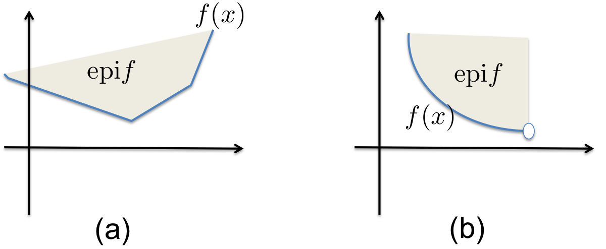
\mathrm{epi}f = \{ ({\boldsymbol{x}},y): {\boldsymbol{x}}\in \mathcal{X}, y \in {\mathbb R}, y\geq f({\boldsymbol{x}}) \}.
The indicator function \iota_{\mathcal{C}}: \mathcal{X}\mapsto [-\infty, \infty] of \mathcal{C}\subset \mathcal{X} is defined as
\iota_{\mathcal{C}}({\boldsymbol{x}}) = \left\{ \begin{array}{ll} 0, & \text{if }{\boldsymbol{x}}\in \mathcal{C}\text{,} \\ \infty, & \text{otherwise.} \end{array} \right.
We often use another definition of the indicator function:
\chi_{\mathcal{C}}({\boldsymbol{x}}) = \left\{ \begin{array}{ll} 1, & \text{if }{\boldsymbol{x}}\in \mathcal{C}\text{,} \\ 0, & \text{otherwise.} \end{array} \right.
The support function of a set \mathcal{C} is defined as
S_{\mathcal{C}}({\boldsymbol{x}}) = \sup\{ \langle {\boldsymbol{x}}, {\boldsymbol{y}}\rangle | {\boldsymbol{y}}\in \mathcal{C}\}.
An affine function is denoted by
{\boldsymbol{x}}\mapsto \mathcal{T}{\boldsymbol{x}}+{\boldsymbol{b}}, \quad {\boldsymbol{x}}\in \mathcal{X}, {\boldsymbol{y}}\in \mathcal{Y}, \mathcal{T}\in \mathcal{B}(\mathcal{X},\mathcal{Y}).
A function f is called lower semicontinuous at {\boldsymbol{x}}_0 if for every \varepsilon>0 there exists a neighbourhood \mathcal{U} of {\boldsymbol{x}}_0 such that f({\boldsymbol{x}}) \geq f({\boldsymbol{x}}_0) -\varepsilon for all {\boldsymbol{x}}\in \mathcal{U}. This is expressed as
\liminf\limits_{{\boldsymbol{x}}\rightarrow {\boldsymbol{x}}_0} f({\boldsymbol{x}}) \geq f({\boldsymbol{x}}_0).
A function is lower semicontinuous if and only if all of its lower level sets \{{\boldsymbol{x}}\in \mathcal{X}: f({\boldsymbol{x}}) \leq \alpha\} are closed. Alternatively, f is lower semicontinuous if and only if the epigraph of f is closed. A function is proper if -\infty \notin f(\mathcal{X}) and \mathrm{dom}f \neq \emptyset.
A self-adjoint operator \mathcal{A}: \mathcal{H}\mapsto \mathcal{H} is positive semidefinite if and only if
\langle {\boldsymbol{x}}, \mathcal{A}{\boldsymbol{x}}\rangle \geq 0, \quad \forall {\boldsymbol{x}}\in \mathcal{H}.
A self-adjoint operator \mathcal{A}: \mathcal{H}\mapsto \mathcal{H} is positive definite if and only if
\langle {\boldsymbol{x}}, \mathcal{A}{\boldsymbol{x}}\rangle > 0, \quad \forall {\boldsymbol{x}}\in \mathcal{H}\setminus\{\mathbf{0}\}.
For simplicity, we denote \mathcal{A}\succeq 0 (resp. \mathcal{A}\succ 0 ) for positive semidefinite (resp. positive definite) operators. If \mathcal{A}:{\mathbb C}^n \mapsto {\mathbb C}^n, then {\mathbb S}^{n}_{++} and {\mathbb S}_{+}^n denote the set of n\times n positive definite and positive semidefinite matrices, respectively. Here, the eigenvalues of positive semidefinite (resp. positive definite) are all real and non-negative (resp. positive).
Convex Sets, Convex Functions
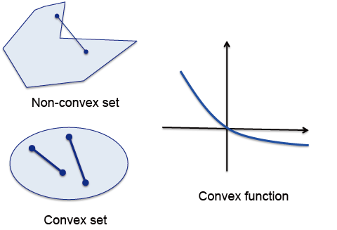
A function f({\boldsymbol{x}}) is a convex function if \mathrm {dom}f is a convex set and
f(\theta {\boldsymbol{x}}_1+ (1-\theta) {\boldsymbol{x}}_2) \leq \theta f({\boldsymbol{x}}_1) + (1-\theta) f({\boldsymbol{x}}_2)
for all {\boldsymbol{x}}_1,{\boldsymbol{x}}_2 \in \mathrm{dom}f, 0\leq \theta \leq 1. A convex set is a set that contains every line segment between any two points in the set (see Figure 3). Specifically, a set \mathcal{C} is convex if { {\boldsymbol{x}}_1,{\boldsymbol{x}}_2 \in \mathcal{C}}, then \theta {\boldsymbol{x}}_1 + (1-\theta){\boldsymbol{x}}_2 \in C for all 0\leq \theta\leq 1. The relation between a convex function and a convex set can also be stated using its epigraph. Specifically, a function f({\boldsymbol{x}}) is convex if and only if its epigraph \mathrm{epi}f is a convex set.
Convexity is preserved under various operations. For example, if \{f_i\}_{i\in I} is a family of convex functions, then, \sup_{i\in I} f_i is convex. In addition, a set of convex functions is closed under addition and multiplication by strictly positive real numbers. Moreover, the limit point of a convergent sequence of convex functions is also convex. Important examples of convex functions are summarized in Table 1.
| Name | f(x) |
|---|---|
| exponential | e^{ax},\quad \forall a \in {\mathbb R} |
| quadratic over linear | x^2/y, \quad (x,y) \in {\mathbb R}\times {\mathbb R}_{++} |
| Huber function | \left\{ \begin{array}{cc} \vert x\vert ^2/2\mu, & \text{if }\vert x\vert <\mu \\ \vert x\vert - \mu/2, & \text{if }\vert x\vert \geq \mu \end{array} \right. |
| relative entropy | y\log y -y \log x, \quad (x,y) \in {\mathbb R}_{++}\times {\mathbb R}_{++} |
| indicator function | \iota_{\mathcal{C}}({\boldsymbol{x}}), \quad \mathcal{C}\text{: convex set} |
| support function | S_{\mathcal{C}}({\boldsymbol{x}}) = \sup\{ \langle {\boldsymbol{x}}, {\boldsymbol{y}}\rangle \vert {\boldsymbol{y}}\in C \} |
| distance to a set | d({\boldsymbol{x}},\mathcal{S}) = \inf_{{\boldsymbol{y}}\in \mathcal{S}} \Vert {\boldsymbol{x}}-{\boldsymbol{y}}\Vert |
| affine function | {\boldsymbol{T}}{\boldsymbol{x}}+ {\boldsymbol{b}}, \quad {\boldsymbol{x}}\in {\mathbb R}^n. |
| quadratic function | {\boldsymbol{x}}^\top {\boldsymbol{Q}}{\boldsymbol{x}}/2, \quad {\boldsymbol{x}}\in {\mathbb R}^n, {\boldsymbol{Q}}\in {\mathbb S}_+ |
| p-norms | \Vert {\boldsymbol{x}}\Vert _p= \left(\sum_i \vert x_i\vert ^p\right)^{1/p}, p \geq 1 |
| l_\infty-norm | \Vert {\boldsymbol{x}}\Vert _\infty = \max_i \vert x_i\vert |
| max function | \max\{x_1,\cdots, x_n\} |
| log-sum-exponential | \log \left(\sum_{i=1}^n e^{x_i} \right), x=(x_1,\cdots, x^{(k)}) \in {\mathbb R}^n. |
| Gaussian data fidelity | \Vert {\boldsymbol{y}}-{\boldsymbol{A}}{\boldsymbol{x}}\Vert ^2, \quad {\boldsymbol{x}}\in \mathcal{H} |
| Poisson data fidelity | \langle \boldsymbol{1}, {\boldsymbol{A}}{\boldsymbol{x}}\rangle - \langle {\boldsymbol{y}}, \log({\boldsymbol{A}}{\boldsymbol{x}}) \rangle,\quad {\boldsymbol{x}}\in {\mathbb R}^n, \boldsymbol{1} =(1,\cdots, 1) \in {\mathbb R}^n |
| spectral norm | \Vert {\boldsymbol{X}}\Vert _2 = \sigma_{\mathrm{max}} ({\boldsymbol{X}}) = (\lambda_{\mathrm{max}} ({\boldsymbol{X}}^\top {\boldsymbol{X}}) )^{1/2}, {\boldsymbol{X}}\in {\mathbb R}^{n\times n} |
| nuclear norm | \Vert {\boldsymbol{X}}\Vert _* = \sum_i\sigma_i ({\boldsymbol{X}}) = \sum_i(\lambda_i ({\boldsymbol{X}}^\top {\boldsymbol{X}}) )^{1/2}, {\boldsymbol{X}}\in {\mathbb R}^{n\times n} |
A function f is concave if -f is convex. It is easy to show that an affine function f({\boldsymbol{x}}) = {\boldsymbol{A}}{\boldsymbol{x}}+{\boldsymbol{b}} is both convex and concave. Examples of concave functions that are often used in this textbook can be found in Table 2.
| Name | f(x) |
|---|---|
| powers | ~~x^p, \quad 0\leq p \leq 1, \quad x \in {\mathbb R}_{++} |
| geometric mean | \left( \prod_{i=1}^n x_i \right)^{\frac{1}{n}} |
| logarithm | \log x, \quad x \in {\mathbb R}_{++} |
| log determinant | \log \det({\boldsymbol{X}}), \quad {\boldsymbol{X}}\in {\mathbb S}_{++} |
Subdifferentials
The directional derivative of f at {\boldsymbol{x}}\in \mathrm{dom}f in the direction of {\boldsymbol{y}}\in \mathcal{H} is defined by
f'({\boldsymbol{x}};{\boldsymbol{y}}) =\lim_{\alpha \downarrow 0} \frac{f({\boldsymbol{x}}+\alpha {\boldsymbol{y}}) - f({\boldsymbol{x}})}{\alpha}\, \tag{28}
if the limit exists. If the limit exists for all {\boldsymbol{y}}\in \mathcal{H}, then one says that f is G\hat{a}teaux differentiable at {\boldsymbol{x}}. Suppose f'({\boldsymbol{x}};\cdot) is linear and continuous on \mathcal{H}. Then, there exist a unique gradient vector \nabla f({\boldsymbol{x}}) \in \mathcal{H} such that
f'({\boldsymbol{x}};{\boldsymbol{y}}) = \langle {\boldsymbol{y}}, \nabla f({\boldsymbol{x}}) \rangle,\quad \forall {\boldsymbol{y}}\in \mathcal{H}.
If a function is differentiable, the convexity of a function can easily be checked using the first- and second-order differentiability, as stated in the following:
Theorem 2 Let f:\mathcal{H}\mapsto (-\infty, \infty] be proper. Suppose that \mathrm{dom}f is open and convex, and f is Gateaux differentiable on \mathrm{dom}f. Then, the following are equivalent:
f is convex.
(First-order): f({\boldsymbol{y}}) \geq f({\boldsymbol{x}}) + \langle {\boldsymbol{y}}-{\boldsymbol{x}}, \nabla f({\boldsymbol{x}}) \rangle, \quad \forall {\boldsymbol{x}}, {\boldsymbol{y}}\in \mathcal{H}.
(Monotonicity of gradient): \langle {\boldsymbol{y}}-{\boldsymbol{x}}, \nabla f({\boldsymbol{y}})- \nabla f({\boldsymbol{x}}) \rangle \geq 0, \quad \forall {\boldsymbol{x}}, {\boldsymbol{y}}\in \mathcal{H}.
Theorem 2 uses the gradient only. When f is twice differentiable there is a second characterisation, and it is usually the one that settles a concrete case.
Theorem 3 Let f be twice differentiable with \mathrm{dom}f open and convex. Then f is convex if and only if its Hessian is positive semidefinite everywhere,
\nabla^2 f({\boldsymbol{x}}) \succeq 0, \qquad \forall {\boldsymbol{x}}\in \mathrm{dom}f . \tag{29}
On the real line this reads f''(x)\geq 0, the familiar test. Two cautions about the strict version. If \nabla^2 f({\boldsymbol{x}}) \succ 0 everywhere then f is strictly convex, but the converse fails: f(x)=x^4 is strictly convex while f''(0)=0. And strict convexity is weaker than strong convexity, which asks for \nabla^2 f({\boldsymbol{x}}) \succeq \mu {\boldsymbol{I}} with \mu>0 — a uniform curvature bound that strict convexity does not provide, and the hypothesis under which gradient descent converges at a linear rate.
As an example, take the quadratic f({\boldsymbol{x}})=\tfrac12 {\boldsymbol{x}}^\top {\boldsymbol{Q}}{\boldsymbol{x}} - {\boldsymbol{b}}^\top{\boldsymbol{x}} with {\boldsymbol{Q}} symmetric. Here \nabla f({\boldsymbol{x}})={\boldsymbol{Q}}{\boldsymbol{x}}-{\boldsymbol{b}} and \nabla^2 f({\boldsymbol{x}})={\boldsymbol{Q}}, so f is convex exactly when {\boldsymbol{Q}}\succeq 0, strongly convex exactly when {\boldsymbol{Q}}\succ 0, and in that case the minimiser is the solution of {\boldsymbol{Q}}{\boldsymbol{x}}={\boldsymbol{b}}. By Equation 15 the eigenvalues of {\boldsymbol{Q}} decide all three questions at once.
If the convergence in Equation 28 is uniform with respect to {\boldsymbol{y}} on bounded sets, i.e.
\lim_{\boldsymbol{0}\neq {\boldsymbol{y}}\rightarrow \boldsymbol{0}} \frac{ f({\boldsymbol{x}}+{\boldsymbol{y}}) - f({\boldsymbol{x}}) - \langle {\boldsymbol{y}}, \nabla f({\boldsymbol{x}}) \rangle}{\|{\boldsymbol{y}}\|} = 0, \tag{30}
then f is Frechet differentiable and \nabla f({\boldsymbol{x}}) is called the Frechet gradient of f at {\boldsymbol{x}}. If f is differentiable and convex, then it is clear that
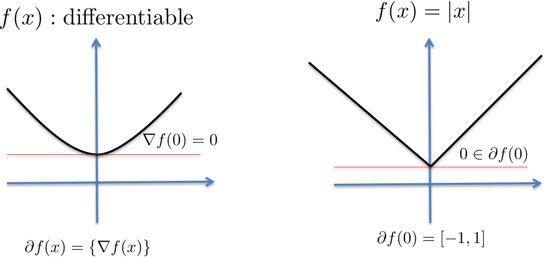
{\boldsymbol{x}}\in \arg\min f \Leftrightarrow \nabla f({\boldsymbol{x}}) = \boldsymbol{0}.
However, if f is not differentiable, we need a more general framework to characterize the minimizers. The sub-differential of f is a set-valued operator defined as
\partial f({\boldsymbol{x}}) = \{{\boldsymbol{u}}\in \mathcal{H}: f({\boldsymbol{y}}) \geq f({\boldsymbol{x}}) + \langle {\boldsymbol{y}}-{\boldsymbol{x}}, {\boldsymbol{u}}\rangle, \quad \forall {\boldsymbol{y}}\in \mathcal{H}\}. \tag{31}
The elements of sub-differential \partial f({\boldsymbol{x}}) are called sub-gradients of f at {\boldsymbol{x}}. Another important role of the subdifferentials comes from Fermat’s rule that characterizes the global minimizers (Figure 4):
Theorem 4 Let f: \mathcal{H}\mapsto (-\infty,\infty] be proper. Then,
\arg\min f=\mathrm{zer}\partial f = \{ {\boldsymbol{x}}\in \mathcal{H}~|~ \boldsymbol{0} \in \partial f({\boldsymbol{x}}) \}. \tag{32}
Convex Conjugate
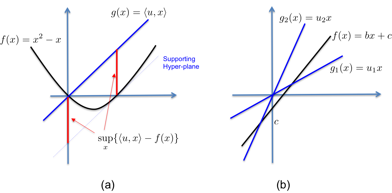
A convex conjugate or convex dual is very important concept for both classical and modern convex optimization techniques. Formally, the conjugate function f^*: \mathcal{H}\mapsto [-\infty,\infty] of a function f: \mathcal{H}\mapsto [-\infty,\infty] is defined as
f^*(u) = \sup_{{\boldsymbol{x}}\in \mathcal{H}} \{\langle {\boldsymbol{u}}, {\boldsymbol{x}}\rangle - f({\boldsymbol{x}})\}. \tag{33}
The transform in Equation 33 is often called Legendre-Fenchel transform.
Figure 5(a) shows a geometric interpretation of the convex conjugate when \mathcal{H}={\mathbb R}. For example, when f(x)=x^2-x, the convex conjugate f^*(u) at u=1 is the maximum difference between g(x)=x and f(x)=x^2-x, which occurs at x=1 in this example. The difference is also equal to the magnitude of the y-intercept of the supporting hyperplane of f(x) at x=1. Figure 5(b) shows another intuitive example. Here, f(x)=bx+c. In this case, the difference between the line g_1(x)=u_1x and f(x) becomes infinite at x\rightarrow -\infty. Similarly, the difference between the line g_2(x)=u_2x and f(x) becomes infinite at x\rightarrow \infty. Only when u=b does the maximum distance become finite, and it is then equal to -c. Therefore, the convex conjugate of f(x)=bx+c is
f^*(u)=\begin{cases} -c, & u=b, \\ \infty, & u\neq b. \end{cases}
Table 3 summarizes these findings for a variety of functions that are often used in biomedical imaging applications.
| f(x) | \mathrm{dom}f | f^*(u) | \mathrm{dom}f^* |
|---|---|---|---|
| f(ax) | D | f^*(u/a) | D |
| f(x+b) | D | f^*(u)-\langle b, u \rangle | D |
| af(x), a>0 | D | a f^*(u/a) | D |
| bx+c | D | \begin{cases}-c, & u=b \\ +\infty, & u\neq b \end{cases} | \{b\} |
| 1/x | {\mathbb R}_{++} | -2 \sqrt{-u} | -{\mathbb R}_{+} |
| -\log x | {\mathbb R}_{++} | -(1+\log(-u)) | -{\mathbb R}_{++} |
| x\log x | {\mathbb R}_{+} | e^{u-1} | {\mathbb R} |
| \sqrt{1+x^2} | {\mathbb R} | -\sqrt{1-u^2} | [-1,1] |
| e^x | {\mathbb R} | u\log(u)-u | {\mathbb R}_+ |
| \log(1+e^x) | {\mathbb R} | u\log(u)+(1-u) \log (1-u) | [0,1] |
| -\log(1-e^x) | {\mathbb R}_{--} | u\log(u)-(1+u) \log (1+u) | {\mathbb R}_+ |
| \frac{\vert x\vert ^p}{p}, ~p>1 | {\mathbb R} | \frac{\vert u\vert ^q}{q},~ \frac{1}{p} + \frac{1}{q} =1 | {\mathbb R} |
| \Vert x\Vert _1 | {\mathbb R}^n | \begin{cases}0, & \Vert u\Vert _\infty\leq 1 \\ \infty & \Vert u\Vert _\infty>1 \end{cases} | \{ u\in {\mathbb R}^n: \Vert u\Vert _\infty\leq 1\} |
| \langle {\boldsymbol{a}}, {\boldsymbol{x}}\rangle+b | {\mathbb R}^n | \begin{cases} - b, & u={\boldsymbol{a}} \\ \infty, & u\neq {\boldsymbol{a}} \end{cases} | \{{\boldsymbol{a}}\} \subset {\mathbb R}^n |
| \frac{1}{2}{\boldsymbol{x}}^\top {\boldsymbol{Q}}{\boldsymbol{x}}, \quad {\boldsymbol{Q}}\in {\mathbb S}_{++} | {\mathbb R}^n | \frac{1}{2}{\boldsymbol{u}}^\top {\boldsymbol{Q}}^{-1}{\boldsymbol{u}} | {\mathbb R}^n |
| \iota_C(x) | C | S_C(u) | \mathcal{H} |
| \log \left(\sum_{i=1}^n e^{x_i} \right) | {\mathbb R}^n | \sum_{i=1}^n u_i \log u_i, \quad \sum_{i=1}^n u_i =1 | {\mathbb R}_{+}^n |
| -\log \det {\boldsymbol{X}}^{-1} | {\mathbb S}_{++}^n | \log \det(-{\boldsymbol{U}})^{-1}-n | -{\mathbb S}_{++}^n |
Here, D\subset \mathcal{H} and we use the interpretation 0\log 0=0. It is clear that f^* is convex since f^* is a point-wise supremum of a convex function of y. In general, if f: \mathcal{H}\mapsto [-\infty,\infty], then the following hold:
For \alpha \in {\mathbb R}_{++}, we have
(\alpha f)^*= \alpha f^*(\cdot/\alpha). \tag{34}
Fenchel–Young inequality:
f({\boldsymbol{x}}) + f^*({\boldsymbol{y}}) \geq \langle {\boldsymbol{y}}, {\boldsymbol{x}}\rangle, \quad \forall {\boldsymbol{x}}, {\boldsymbol{y}}\in \mathcal{H}. \tag{35}
Let f,g be proper functions from \mathcal{H} to (-\infty,\infty]. Then,
f({\boldsymbol{x}})+g({\boldsymbol{x}}) \geq -f^*({\boldsymbol{u}})-g^*(-{\boldsymbol{u}}),\quad \forall {\boldsymbol{x}},{\boldsymbol{u}}\in \mathcal{H}. \tag{36}
If f is convex, proper, and lower semicontinuous, then the following properties hold:
\begin{aligned} f^{**} &= f, \\ {\boldsymbol{y}}\in \partial f({\boldsymbol{x}}) &\Longleftrightarrow& f({\boldsymbol{x}})+ f^*({\boldsymbol{y}})= \langle {\boldsymbol{x}}, {\boldsymbol{y}}\rangle \Longleftrightarrow {\boldsymbol{x}}\in \partial f^*({\boldsymbol{y}}). %\\ %(\partial f)^{-1} &= \partial f^* \end{aligned} \tag{37}
Lagrangian Dual Formulation
Perhaps one of the most important uses of convex conjugate is to obtain the dual formulation. More specifically, for a given primal problem (P),
(P) : \quad \min_{{\boldsymbol{x}}\in \mathcal{H}}f({\boldsymbol{x}})+g({\boldsymbol{x}}),
we can obtain the associated dual problem using Equation 36:
(D): \quad -\min_{{\boldsymbol{u}}\in \mathcal{H}} f^*({\boldsymbol{u}})+ g^*(-{\boldsymbol{u}}).
The gap between the primal and dual problem is called the duality gap.
Example 2 (Dual for Composite Function) For the given primal problem:
(P) : \quad \min\limits_{{\boldsymbol{x}}\in {\mathbb R}^n}f({\boldsymbol{x}})+g({\boldsymbol{A}}{\boldsymbol{x}}), \tag{38}
with {\boldsymbol{A}}\in {\mathbb R}^{m\times n}, the dual problem is given by
(D): -\min_{{\boldsymbol{u}}\in {\mathbb R}^m} f^*({\boldsymbol{A}}^\top {\boldsymbol{u}})+ g^*(-{\boldsymbol{u}}).
Proof. Note that (P) is equivalent to the following constraint minimization problem:
\begin{aligned} \min\limits_{{\boldsymbol{x}},{\boldsymbol{y}}} & f({\boldsymbol{x}})+g({\boldsymbol{y}})\\ \text{subject to} & {\boldsymbol{A}}{\boldsymbol{x}}={\boldsymbol{y}}, \end{aligned}
which provides
\begin{aligned} \min\limits_{{\boldsymbol{x}}\in {\mathbb R}^n}f({\boldsymbol{x}})+g({\boldsymbol{A}}{\boldsymbol{x}})&\geq \min\limits_{{\boldsymbol{x}},{\boldsymbol{y}}} f({\boldsymbol{x}})+g({\boldsymbol{y}}) +{\boldsymbol{u}}^\top({\boldsymbol{A}}{\boldsymbol{x}})-{\boldsymbol{u}}^\top {\boldsymbol{y}}\\ &= \min_{\boldsymbol{x}}\{f({\boldsymbol{x}})+({\boldsymbol{A}}^\top {\boldsymbol{u}})^\top {\boldsymbol{x}}\} + \min_{\boldsymbol{y}}\{g({\boldsymbol{y}})-{\boldsymbol{u}}^\top {\boldsymbol{y}}\}\\ &= -f^*(-{\boldsymbol{A}}^\top {\boldsymbol{u}})-g^*({\boldsymbol{u}}), \end{aligned}
where the first line drops the constraint {\boldsymbol{A}}{\boldsymbol{x}}={\boldsymbol{y}}, so the relaxation is a lower bound for every {\boldsymbol{u}}, and the second line holds with equality because the minimisation separates in {\boldsymbol{x}} and {\boldsymbol{y}}.
Since this holds for every {\boldsymbol{u}}, taking the supremum gives
\max_{{\boldsymbol{u}}\in {\mathbb R}^m} -f^*(-{\boldsymbol{A}}^\top {\boldsymbol{u}})-g^*({\boldsymbol{u}}) = -\min_{{\boldsymbol{u}}\in {\mathbb R}^m} f^*(-{\boldsymbol{A}}^\top {\boldsymbol{u}})+ g^*({\boldsymbol{u}}),
and substituting {\boldsymbol{u}}\leftarrow -{\boldsymbol{u}} yields the dual problem
-\min_{{\boldsymbol{u}}\in {\mathbb R}^m} f^*({\boldsymbol{A}}^\top {\boldsymbol{u}})+ g^*(-{\boldsymbol{u}}).
This concludes the proof.
Example 3 (Quadratic Programming under Affine Constraint) Consider the following optimization problem:
P: \min \frac{1}{2} {\boldsymbol{x}}^\top {\boldsymbol{x}}\quad \text{subject to}\quad {\boldsymbol{b}}={\boldsymbol{A}}{\boldsymbol{x}}
with {\boldsymbol{A}}\in {\mathbb R}^{m\times n}. Now, we define \mathcal{C}=\{\boldsymbol{0}\} such that {\boldsymbol{b}}-{\boldsymbol{A}}{\boldsymbol{x}}\in \mathcal{C}. Then, the original minimization problem becomes
\begin{aligned} \min\limits_{{\boldsymbol{x}},{\boldsymbol{y}}} & \iota_{\mathcal{C}}({\boldsymbol{y}})+\frac{1}{2}{\boldsymbol{x}}^\top {\boldsymbol{x}}\\ \text{subject to} & {\boldsymbol{y}}={\boldsymbol{b}}-{\boldsymbol{A}}{\boldsymbol{x}}. \end{aligned}
Therefore, we have
\begin{aligned} \min\limits_{{\boldsymbol{x}}} \iota_{\mathcal{C}}({\boldsymbol{b}}-{\boldsymbol{A}}{\boldsymbol{x}})+\frac{1}{2}{\boldsymbol{x}}^\top {\boldsymbol{x}}&\geq \min_{{\boldsymbol{x}},{\boldsymbol{y}}} \iota_{\mathcal{C}}({\boldsymbol{y}})+\frac{1}{2}{\boldsymbol{x}}^\top {\boldsymbol{x}}+{\boldsymbol{u}}^\top({\boldsymbol{b}}-{\boldsymbol{A}}{\boldsymbol{x}}-{\boldsymbol{y}}) \\ &\geq \min_{{\boldsymbol{y}}} \iota_{\mathcal{C}}({\boldsymbol{y}})-{\boldsymbol{u}}^\top {\boldsymbol{y}}+ \min_{\boldsymbol{x}}\frac{1}{2}{\boldsymbol{x}}^\top {\boldsymbol{x}}-{\boldsymbol{u}}^\top {\boldsymbol{A}}{\boldsymbol{x}}+{\boldsymbol{u}}^\top {\boldsymbol{b}}\\ &\geq \min_{{\boldsymbol{y}}\in \{\boldsymbol{0}\}}-{\boldsymbol{u}}^\top {\boldsymbol{y}}+ \min_{\boldsymbol{x}}\frac{1}{2}{\boldsymbol{x}}^\top {\boldsymbol{x}}-{\boldsymbol{u}}^\top {\boldsymbol{A}}{\boldsymbol{x}}+{\boldsymbol{u}}^\top {\boldsymbol{b}}\\ &= -\frac{1}{2}{\boldsymbol{u}}^\top {\boldsymbol{A}}{\boldsymbol{A}}^\top {\boldsymbol{u}}+ {\boldsymbol{u}}^\top {\boldsymbol{b}}, \end{aligned}
where the last equality comes from {\boldsymbol{x}}={\boldsymbol{A}}^\top {\boldsymbol{u}} at the minimizer. Hence, the dual problem becomes
D: \min_{{\boldsymbol{u}}\in{\mathbb R}^m} \frac{1}{2}{\boldsymbol{u}}^\top {\boldsymbol{A}}{\boldsymbol{A}}^\top {\boldsymbol{u}}- {\boldsymbol{u}}^\top {\boldsymbol{b}}.
Why is this dual formulation useful? Suppose that {\boldsymbol{A}} is highly ill-posed, say that n=1000 and m=1. Then, the dual problem (D) is a one-dimensional problem which is computationally much less expensive than the primal problem (P) of the dimension n=1000. After the dual solution \hat {\boldsymbol{u}} is obtained, the primal solution is just \hat {\boldsymbol{x}}={\boldsymbol{A}}^\top\hat {\boldsymbol{u}}.
We formally define a Lagrangian dual problem.
Definition 16 Suppose that a primal problem is given by
\begin{aligned} \min_{\boldsymbol{x}}& f_0({\boldsymbol{x}}) &\\ \mathrm{subject~to} & f_i({\boldsymbol{x}})\leq 0,& i=1,\cdots, n, \\ &h_i({\boldsymbol{x}})=0,& i=1,\cdots, p. \end{aligned}
Then, the associated Lagrangian dual problem is defined by
\begin{aligned} {\max_{{\boldsymbol {\alpha}},{\boldsymbol{\nu}}}}& g({\boldsymbol {\alpha}},{\boldsymbol{\nu}}) & \\ \mathrm{subject~to} & {\boldsymbol {\alpha}}\geq \mathbf{0}, \end{aligned}
where {\boldsymbol {\alpha}}=[\alpha_1,\cdots,\alpha_n] and {\boldsymbol{\nu}}=[\nu_1,\cdots,\nu_p] are referred to as the dual variables or Lagrangian multipliers, {\boldsymbol {\alpha}}\geq \mathbf{0} implies that each element is non-negative, and the Lagrangian dual function g({\boldsymbol {\alpha}},{\boldsymbol{\nu}}) is defined by
\begin{aligned} {g({\boldsymbol {\alpha}}, {\boldsymbol{\nu}})} := \inf_{\boldsymbol{x}}\left\{ f_0({\boldsymbol{x}}) + \sum_{i=1}^n \alpha_i f_i({\boldsymbol{x}}) + \sum_{j=1}^p \nu_jh_j({\boldsymbol{x}})\right\}. \end{aligned}
Two properties hold with no assumption on the primal problem at all. First, g is concave, being a pointwise infimum of functions that are affine in ({\boldsymbol {\alpha}},{\boldsymbol{\nu}}) — so the dual problem is a concave maximisation, hence convex, even when the primal is not. Second, weak duality: for any feasible {\boldsymbol{x}} and any {\boldsymbol {\alpha}}\geq \mathbf{0},
g({\boldsymbol {\alpha}},{\boldsymbol{\nu}}) \;\leq\; f_0({\boldsymbol{x}}) + \sum_{i=1}^n \alpha_i f_i({\boldsymbol{x}}) + \sum_{j=1}^p \nu_j h_j({\boldsymbol{x}}) \;\leq\; f_0({\boldsymbol{x}}) , \tag{39}
where the first inequality is the definition of the infimum and the second holds because \alpha_i f_i({\boldsymbol{x}})\leq 0 and h_j({\boldsymbol{x}})=0 at a feasible {\boldsymbol{x}}. Taking the best on each side gives d^\star \leq p^\star, and the difference p^\star - d^\star \geq 0 is the duality gap. This is what makes the dual useful even when it is not tight: any feasible dual point certifies a lower bound on the primal optimum.
One of the important findings in convex optimization theory is that if the primal problem is convex and a constraint qualification holds — for example Slater’s condition, which asks that some strictly feasible point exist, i.e. a point {\boldsymbol{x}} with f_i({\boldsymbol{x}})<0 for all i and h_j({\boldsymbol{x}})=0 for all j — then we have the following strong duality:
\begin{aligned} g({\boldsymbol {\alpha}}^*,{\boldsymbol{\nu}}^*)=f_0({\boldsymbol{x}}^*), \end{aligned} \tag{40}
where {\boldsymbol{x}}^* and {\boldsymbol {\alpha}}^*,{\boldsymbol{\nu}}^* are the optimal solutions for the primal and dual problems, respectively. i.e. the duality gap is zero. Often, the dual formulation is easier to solve than the primal problem.
When strong duality holds and the functions are differentiable, the primal and dual optima are characterised by the Karush–Kuhn–Tucker conditions: at {\boldsymbol{x}}^* and ({\boldsymbol {\alpha}}^*,{\boldsymbol{\nu}}^*),
\begin{aligned} f_i({\boldsymbol{x}}^*) &\leq 0, \quad h_j({\boldsymbol{x}}^*) = 0 && \text{(primal feasibility)},\\ \alpha_i^* &\geq 0 && \text{(dual feasibility)},\\ \alpha_i^* f_i({\boldsymbol{x}}^*) &= 0 && \text{(complementary slackness)},\\ \nabla f_0({\boldsymbol{x}}^*) + \sum_i \alpha_i^* \nabla f_i({\boldsymbol{x}}^*) + \sum_j \nu_j^* \nabla h_j({\boldsymbol{x}}^*) &= \mathbf{0} && \text{(stationarity)}. \end{aligned} \tag{41}
Complementary slackness is the informative one: a constraint that is inactive at the optimum carries a zero multiplier, so the multipliers say which constraints are actually binding. For a convex problem satisfying Slater’s condition the KKT conditions are necessary and sufficient, which turns a constrained problem into a system of equations and inequalities. Note that stationarity is the constrained analogue of \nabla f = \mathbf{0}, and that Fermat’s rule of the subdifferential section generalises it to the non-differentiable case.
There is also an interesting geometric interpretation, which will be explained later in this book.
Written by Jong Chul Ye.