3 StyleGAN, Normalization, Attention, and Image Translation
3.1 Overview
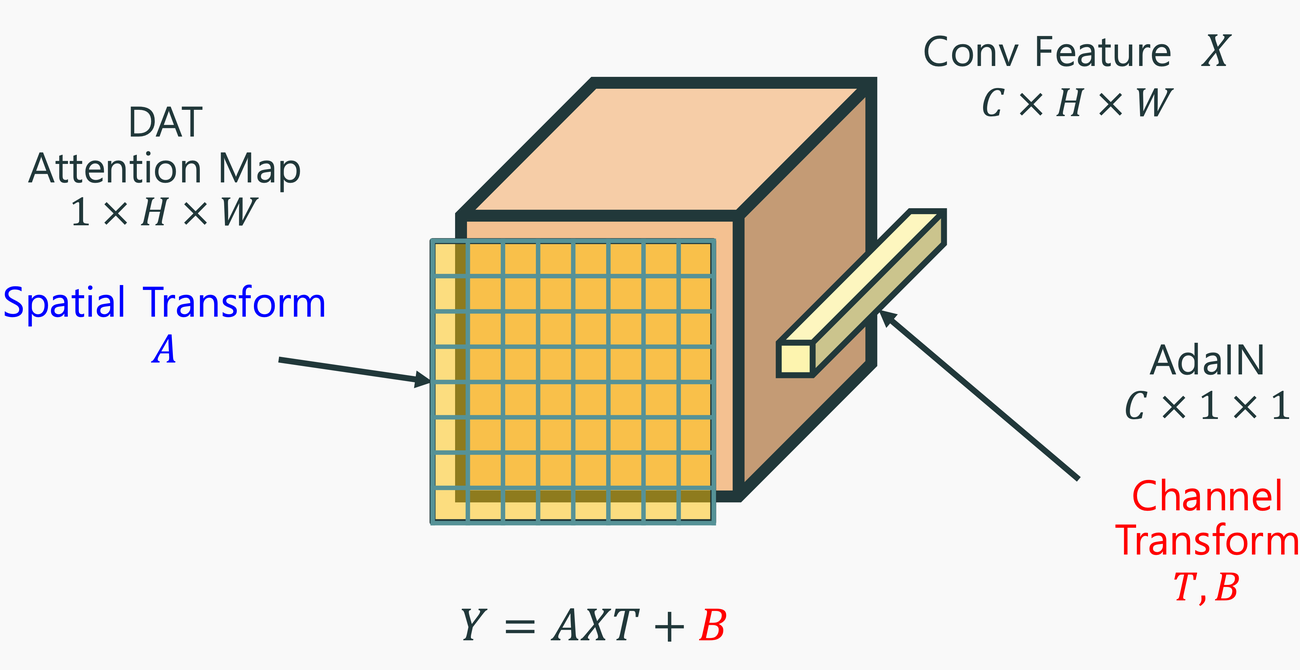
Earlier GAN lectures asked how a discriminator measures mismatch between real and generated distributions. This lecture asks a different question: where should a generator receive information so that we can control what it generates? The lecture moves from feature normalization and attention, through StyleGAN and content-style disentanglement, to paired, unpaired, and multi-domain image translation. The organizing equation is Y=AXT+B: left multiplication acts on spatial positions, while right multiplication acts on channels.
The main exposition follows Part 1 - GAN, pp. 78–125, and the accompanying lecture transcript (Ye 2026a, 2026b). Paper-level equations are added where they clarify a model discussed in class. A section of advanced topics at the end collects the material that was not developed in the provided pp. 78–125/script, so that the main narrative follows the class itself.
Color key. \textcolor{blue}{\text{Blue}} marks spatial/content control; \textcolor{red}{\text{red}} marks style/channel control; \textcolor{violet}{\text{violet}} marks reconstruction or consistency; \textcolor{teal}{\text{teal}} marks domain supervision; and \textcolor{orange}{\text{orange}} marks diversity. Shared adversarial terms remain black. Labels accompany color so that the comparisons remain readable in grayscale.
3.2 Notation
| Symbol | Meaning |
|---|---|
| N=HW, C, M | Spatial positions, feature channels, and minibatch size |
| X=[x_1,\ldots,x_C]\in\mathbb{R}^{N\times C} | One image’s feature matrix; x_c is a spatial channel map |
| x^n\in\mathbb{R}^{1\times C} | Row of X: channel features at position n |
| \mathbf 1_N, I_N, \operatorname{diag}(v) | All-ones vector, identity matrix, diagonal matrix |
| \mu_X, \Sigma_X | Channel mean vector and centered channel covariance |
| x\sim p_{\mathcal{X}}, y\sim p_{\mathcal{Y}} | Images from two domains, distinct from feature matrix X |
| G, F, D | Generators and discriminator; each section states their domains |
| z, w, s | Prior latent, mapped latent, and style code |
| k, t, K | Source domain, target domain, number of domains |
| T_\#p | Push-forward: the distribution of T(u) when u\sim p |
Unless stated otherwise, expectations are over the displayed data and independently sampled latent variables. Empirical variances use divisor N, not N-1, matching the lecture. Formulas assume positive variances; implementations add \epsilon>0 under square roots. Norm subscripts distinguish the vector L_1/L_2 norms from the matrix Frobenius norm \|\cdot\|_F.
3.3 Normalization as channel-wise transformation
3.3.1 What is averaged in batch, layer, and instance normalization?
For a minibatch tensor X_{mnc}, normalization has the common form
Y_{mnc}=\gamma\frac{X_{mnc}-\mu}{\sqrt{v+\epsilon}}+\beta. \tag{3.1}
The important difference is not this formula, but which entries share its statistics. The following table uses the CNN layer-normalization convention on slide 87, which pools spatial positions and channels within one image (Ye 2026a, 83–88; Ioffe and Szegedy 2015; Ba et al. 2016; Ulyanov et al. 2016).
| Method | Mean; variance uses the same averaging set | Shared over | Main benefit / limitation |
|---|---|---|---|
| Batch normalization (BN) | \mu_c=\frac{1}{MN}\sum_{m,n}X_{mnc} | Batch and positions, separately per channel | Useful optimization conditioning; batch-dependent estimates and train/test statistics can differ |
| Layer normalization (LN) | \mu_m=\frac{1}{NC}\sum_{n,c}X_{mnc} | All features of one image | Independent of batch size; this choice does not standardize each channel separately |
| Instance normalization (IN) | \mu_{mc}=\frac1N\sum_nX_{mnc} | Positions of one image and channel | Removes per-image channel contrast; may discard useful absolute intensity information |
For each table row, v is the average of (X-\mu)^2 over the indicated indices. BN and IN use channel-specific learned \gamma_c,\beta_c. Slide 87 simplifies LN to shared scalar gain and bias; the original LN paper also allows neuron-wise gains and biases. Transformer token-wise LN is another axis choice: it normalizes channels within each token, not all positions in an image. These choices should not be silently interchanged.
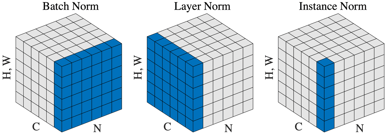
BN uses minibatch statistics during training and population estimates at inference. IN recomputes statistics separately for each image; LN also avoids dependence on other minibatch samples. The transcript initially describes BN statistics as channel-independent but then explicitly corrects this: \mu_c and v_c depend on the channel (Ye 2026b).
3.3.2 Deriving the matrix representation
Suppress the batch index. Set \sigma_c=\sqrt{v_c+\epsilon}, \mu=(\mu_1,\ldots,\mu_C)^\top, and \beta=(\beta_1,\ldots,\beta_C)^\top. Expanding each normalized channel gives
\begin{aligned} y_c&=\frac{\gamma_c}{\sigma_c}x_c+ \left(\beta_c-\frac{\gamma_c\mu_c}{\sigma_c}\right)\mathbf1_N,\\ Y&=X\,\textcolor{red}{T}+B,\\ T&=\operatorname{diag}(\gamma_1/\sigma_1,\ldots,\gamma_C/\sigma_C),\qquad B=\mathbf1_N(\beta^\top-\mu^\top T). \end{aligned} \tag{3.2}
This is the lecture’s Y=XT+B representation. A diagonal T rescales channels; a dense T can mix them. Neither directly routes a value from one spatial position to another. For IN the matrices depend on the current image; for BN they also depend on the minibatch. Thus this is an affine representation conditional on the computed statistics, not a claim that the complete normalization operation is a fixed affine function of X.
3.4 Style transfer: statistics, AdaIN, and transport
3.4.1 Adaptive instance normalization
For content features X and reference-style features S, AdaIN replaces learned fixed IN gains and biases by reference statistics (Huang and Belongie 2017, secs. 3–4; Ye 2026a, 80, 89–90):
\begin{aligned} \operatorname{AdaIN}(x_c,s_c) &=\textcolor{red}{\sigma_{S,c}}\, \frac{x_c-\mu_{X,c}\mathbf1_N}{\sigma_{X,c}} +\textcolor{red}{\mu_{S,c}}\mathbf1_N,\\ Y&=(X-\mathbf1_N\mu_X^\top) \textcolor{red}{D_X^{-1}D_S}+\mathbf1_N\mu_S^\top, \quad D_X=\operatorname{diag}(\sigma_X). \end{aligned} \tag{3.3}
D_S is defined similarly; X and S need not have the same number of positions. A fixed encoder, this transform, and a learned decoder produce a stylized image. The decoder is trained using content-feature and style-statistic losses. Reference statistics are computed from S, not new free parameters trained for every reference image.
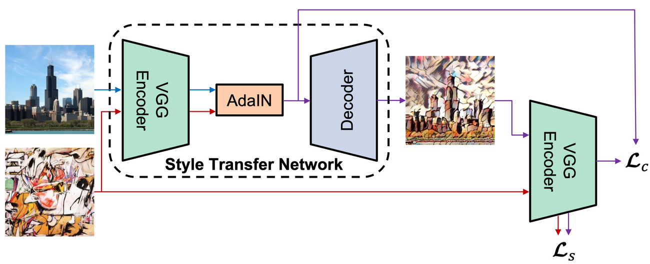
Advantage: efficient arbitrary-reference stylization without an eigendecomposition. Limitation: channel means and variances do not determine cross-channel covariance or a general feature distribution. A successful feature transform also need not invert perfectly through the decoder.
3.4.2 Why AdaIN resembles Gaussian optimal transport
The lecture connects AdaIN to Gaussian optimal transport (Ye 2026a, 40, 80; 2026b). Here is the missing one-dimensional derivation. Let U\sim\mathcal{N}(\mu_u,\sigma_u^2) and V\sim\mathcal{N}(\mu_v,\sigma_v^2), with positive standard deviations. For squared Euclidean transport cost, the increasing quantile map is
\begin{aligned} \mathcal T(u) &=F_V^{-1}(F_U(u))\\ &=\mu_v+\sigma_v\Phi^{-1}\left(\Phi\left(\frac{u-\mu_u}{\sigma_u}\right)\right)\\ &=\mu_v+\frac{\sigma_v}{\sigma_u}(u-\mu_u). \end{aligned} \tag{3.4}
\Phi is the standard normal CDF. Consequently, \mathbb{E}[\mathcal T(U)]=\mu_v and \operatorname{Var}[\mathcal T(U)]=\sigma_v^2. For Gaussian channel vectors with diagonal covariance and separable squared cost, applying this map coordinate-wise gives AdaIN. The channels may have different means and variances: independence, rather than identical distributions across channels, is the relevant condition.
For positive-definite full covariances, the Gaussian squared-cost map for column vectors is instead
\mathcal T(u)=\mu_S+M(u-\mu_X),\quad M=\Sigma_X^{-1/2} (\Sigma_X^{1/2}\Sigma_S\Sigma_X^{1/2})^{1/2} \Sigma_X^{-1/2}. \tag{3.5}
Thus the lecture’s OT interpretation is exact under a Gaussian/diagonal model, not a theorem that empirical CNN features are Gaussian or that AdaIN transports their complete non-Gaussian distributions optimally.
3.4.3 Whitening and coloring transform
WCT extends channel-wise scaling to full channel covariance (Li et al. 2017, sec. 3.2; Ye 2026a, 91). With X_c=X-\mathbf1_N\mu_X^\top and \Sigma_X=X_c^\top X_c/N, write \Sigma_X=U_X\Lambda_XU_X^\top and similarly for S. In the lecture’s row-vector convention,
Y=X_c\,\textcolor{red}{\Sigma_X^{-1/2}\Sigma_S^{1/2}} +\mathbf1_N\mu_S^\top. \tag{3.6}
The covariance calculation makes the two steps explicit:
\begin{aligned} \operatorname{Cov}(X_c\Sigma_X^{-1/2})&=I_C,\\ \operatorname{Cov}(Y)&= \Sigma_S^{1/2}\Sigma_X^{-1/2}\Sigma_X\Sigma_X^{-1/2}\Sigma_S^{1/2} =\Sigma_S. \end{aligned} \tag{3.7}
Advantage: matches correlations that diagonal AdaIN ignores. Limitation: forming a covariance costs O(NC^2) and a dense eigendecomposition costs O(C^3); small eigenvalues need regularization or truncation. Exact full-rank matching assumes positive-definite covariances.
Clarification of the slide: the covariance is centered and the mean correction is B=\mathbf1_N\mu_S^\top-\mathbf1_N\mu_X^\top T, not a channel-wise diagonal expression copied unchanged from AdaIN. WCT is a valid covariance-matching transport, but it is generally not the squared-cost optimal map in Equation 3.5. They coincide in the diagonal, or more generally commuting-covariance, case.
3.5 Attention: transformation along the other axis
3.5.1 Queries, keys, and values
A spatial attention layer combines rows rather than columns. A query represents what an output position seeks, a key supplies matching information, and a value is the information to be aggregated. With W_Q,W_K\in\mathbb{R}^{C\times d} and W_V\in\mathbb{R}^{C\times d_v}, set Q=XW_Q, K=XW_K, and V=XW_V. The output is (Ye 2026a, 92–95; Vaswani et al. 2017)
\begin{aligned} a_{mn}&=\frac{\exp(\operatorname{score}(q^m,k^n))} {\sum_{j=1}^N\exp(\operatorname{score}(q^m,k^j))},\\ y^m&=\sum_{n=1}^Na_{mn}v^n,\qquad Y=\textcolor{blue}{A}XW_V. \end{aligned} \tag{3.8}
The lecture lists dot-product, scaled dot-product, and cosine scores:
qk^\top,\qquad \frac{qk^\top}{\sqrt d},\qquad \frac{qk^\top}{\|q\|_2\|k\|_2}.
For a fixed query index m, \sum_na_{mn}=1: rows of A sum to one. The exponential normalization is softmax, not the sigmoid mentioned hesitantly in the transcript. W_Q,W_K,W_V are learned linear projections; the attention layer becomes nonlinear through its data-dependent weights. In cross-attention, queries and key/value features can come from different inputs, giving a generally rectangular A.
Advantage: dense attention provides direct long-range interaction. Limitation: explicitly forming self-attention requires O(N^2) weights; that cost grows rapidly with image resolution. The value projection changes the channel representation, but does not itself standardize a mean or variance.
3.5.2 The unified transform and its limits
The lecture collects these operations as
\boxed{Y=\underbrace{\textcolor{blue}{A}}_{\text{spatial axis}} X\underbrace{\textcolor{red}{T}}_{\text{channel axis}}+B.} \tag{3.9}
At index level, Y_{nc}=\sum_{m,j}A_{nm}X_{mj}T_{jc}+B_{nc}. Reading the two sums separately is what distinguishes the mechanisms. The sum over m runs over input positions, so a dense A gathers many positions into one output position while a diagonal A only gates each position in place. The sum over j runs over input channels, so a dense T mixes channels while a diagonal T rescales each one across every position at once.
The point of writing it this way is that the operations of this chapter are not four unrelated mechanisms but four choices of which factor is active and where it is computed from (Ye 2026a, 96–97):
| Operation | Form | A | T | computed from |
|---|---|---|---|---|
| Instance norm, AdaIN, WCT | Y=XT+B | I | channel mixing or scaling | X, and a style input for AdaIN and WCT |
| Self-attention | Y=AX | dense, position mixing | I | X alone |
| Cross-attention | Y=AX | dense, generally rectangular | I | queries from X, keys and values from another input |
| Channel attention (SENet) | Y=XT | I | diagonal | X, pooled over position |
Two rows in Table 3.1 are worth separating because they are easy to conflate. Channel attention (Hu et al. 2018) and AdaIN both act through a diagonal T, but AdaIN’s scale comes from a style image and SENet’s comes from the same feature map pooled over position — the first imports information, the second redistributes it. And self- and cross-attention differ only in where the keys come from, which is the whole of the step from a generator that stylises one image to the translation models of Section 3.7.
The lecturer’s word dual describes complementary tensor axes, not optimization duality. For fixed T, \operatorname{col}(XT)\subseteq\operatorname{col}(X); for fixed A, \operatorname{row}(AX)\subseteq\operatorname{row}(X). However, statistics-dependent A,T,B must be recomputed when their inputs change. Associativity (AX)T=A(XT) for fixed matrices does not imply that complete normalization and attention layers commute, or that separate axes guarantee independent semantic factors.
3.6 Generators with style and content control
Here disentanglement means being able to vary one designated group of attributes while holding another approximately fixed. The lecture associates content with pose, geometry, and expression, and style with appearance and sometimes identity (Ye 2026a, 104–13). This is an operational convention, not a universal taxonomy.
3.6.1 StyleGAN: learned styles and stochastic detail
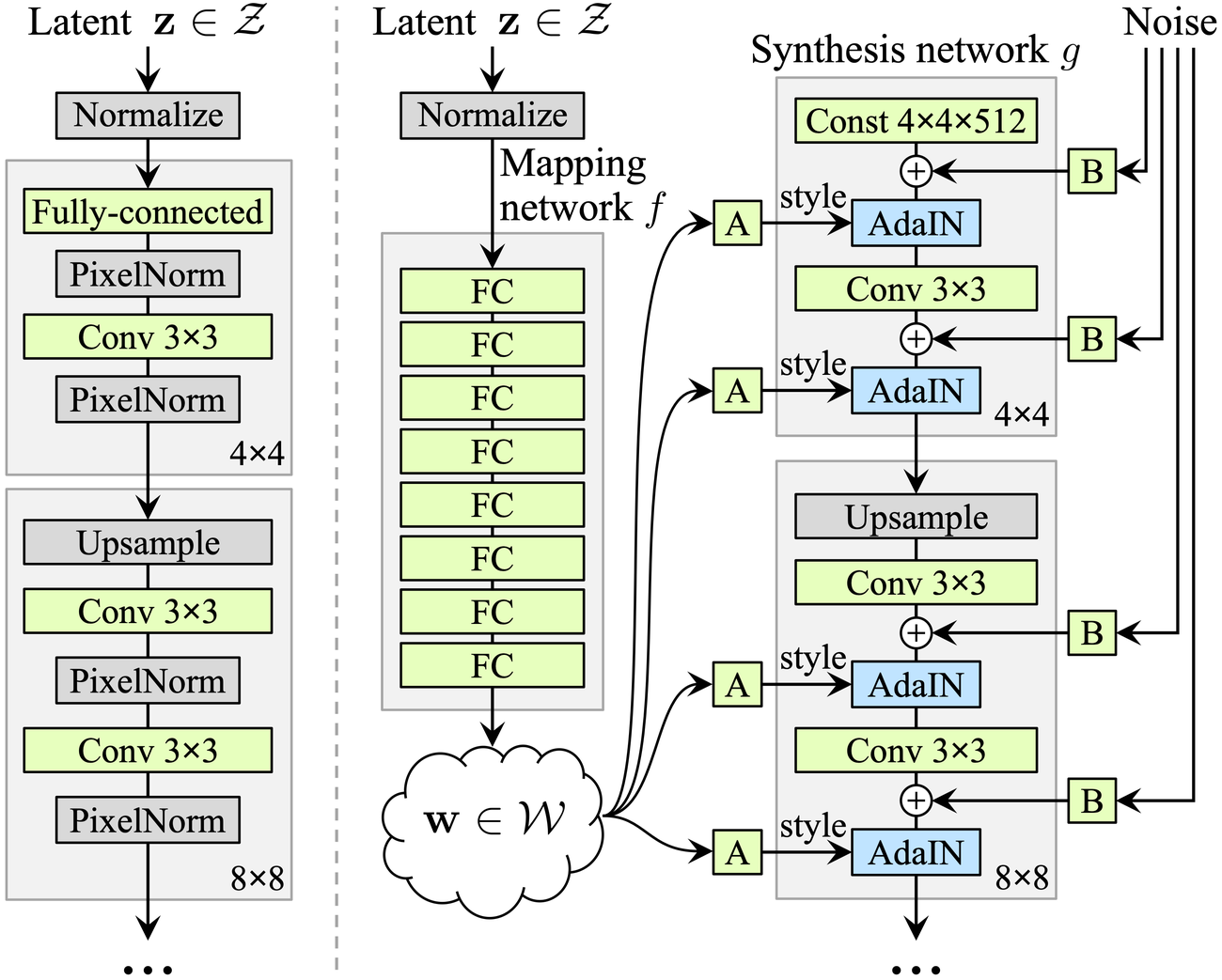
StyleGAN starts from a learned 4\times4\times512 constant tensor shared across generated samples. An eight-layer mapping MLP produces w=f(z)\in\mathcal{W} from z\sim\mathcal{N}(0,I); layer-specific affine maps produce style parameters (Karras et al. 2019, secs. 2–3; Ye 2026a, 79, 101–3). A synthesis stage can be summarized as
\begin{aligned} h_\ell&=\operatorname{Conv}_\ell(\operatorname{Up}(X_{\ell-1})),\\ u_{\ell c}&=\rho(h_{\ell c}+\textcolor{blue}{b_{\ell c}n_\ell}+a_{\ell c}),\\ X_{\ell c}&=\textcolor{red}{\gamma_{\ell c}(w)} \frac{u_{\ell c}-\mu(u_{\ell c})}{\sigma(u_{\ell c})} +\textcolor{red}{\beta_{\ell c}(w)}, \qquad (\gamma_\ell,\beta_\ell)=L_\ell(w). \end{aligned} \tag{3.10}
Here n_\ell is a spatial Gaussian noise map shared across channels with learned channel scales b_{\ell c}; \rho is the nonlinearity. Upsampling is omitted at layers that retain resolution. Unlike reference-based AdaIN, style parameters are predicted from w; a predicted gain need not be a positive reference standard deviation.
Why use \mathcal{W}? The mapping can reshape the simple prior before synthesis, rather than forcing all semantic variation to follow its geometry directly. The paper measures improved disentanglement using perceptual path length and linear separability; this is empirical, not guaranteed. Style mixing uses different w values before and after a selected layer. Resampling noise mainly changes stochastic detail, not a controlled semantic attribute.
Advantage: scale-specific control with high-resolution synthesis. Limitation: styles can still change pose and geometry, so style is broader than texture; complete content-style separation is absent. Its contribution is architectural, not a new GAN divergence.
3.6.2 Structured noise injection: structured content at the input
SNI replaces the fixed input by a tensor assembled from location-specific mappings. A schematic form of its local/shared construction is (Alharbi and Wonka 2020, secs. 3–4)
X_0^{r}=\textcolor{blue}{P_r[z_r^{\mathrm{local}};z_{g(r)}^{\mathrm{region}};z^{\mathrm{global}}]+b_r}, \qquad (\gamma_\ell,\beta_\ell)=\textcolor{red}{L_\ell(f_s(z_s))}. \tag{3.11}
r indexes input-grid cells and g(r) their shared region. Separate P_r restrict which local latent affects each cell. The paper’s preferred configuration uses an 8\times8 local grid, shared 2\times2 region codes, and one global code; the lecture’s 4\times4 drawing is a simplified architecture, not its only setting. Style modulation begins later in the preferred configuration.
Advantage: local, regional, and global control without attribute labels. Limitation: content enters through the initial grid, while style can enter at many layers. Spatial leakage and remaining entanglement depend on grid/code design; changing background style may also change the foreground. The lecture calls this asymmetry the motivation for hierarchical DAT (Ye 2026a, 105).
3.6.3 Diagonal GAN: hierarchical spatial gating
Diagonal GAN introduces content control at several resolutions alongside style control (Kwon and Ye 2021, secs. 3–4; Ye 2026a, 104–13). With independent content and style latents, the paper’s residual diagonal attention is
\begin{aligned} c&=f_c(z_c),\quad s=f_s(z_s),\quad d_\ell=\operatorname{sigmoid}(M_\ell(c)),\\ \textcolor{blue}{A_\ell(c)}&=I+\textcolor{blue}{\eta_\ell\operatorname{diag}(d_\ell)},\\ \widetilde X_\ell&=\textcolor{blue}{A_\ell(c)}X_\ell, \qquad Y_\ell=\operatorname{AdaIN}(\widetilde X_\ell,\textcolor{red}{s}). \end{aligned} \tag{3.12}
\eta_\ell denotes the paper’s learned coefficient \beta, renamed to avoid confusing it with AdaIN’s shift. This is not dense query-key attention: every channel receives the same spatial gate. AdaIN’s statistics are computed on its actual incoming tensor \widetilde X_\ell.
The paper also adds a diversity-sensitive term, often omitted by the slides:
\mathcal{L}_{\mathrm{DS}}=\mathbb{E}\left[ \textcolor{orange}{\max\{\tau-\|G(z_s,z_c^1)-G(z_s,z_c^2)\|_1,0\}} \right],\qquad \mathcal{L}_G=\mathcal{L}_{G,\mathrm{adv}}+\mathcal{L}_{\mathrm{DS}}. \tag{3.13}
The shared style is fixed while content varies. Once the distance exceeds \tau, this term stops rewarding further separation; it does not enforce a hard upper bound on the distance. Training uses non-saturating adversarial loss and R_1 discriminator regularization.
Advantage: spatial control at coarse and fine resolutions with O(N) gate values. Limitation: a diagonal gate does not itself move pixels; geometric changes emerge through subsequent convolutions. Separation is an empirical inductive bias, not a theorem of perfect disentanglement.
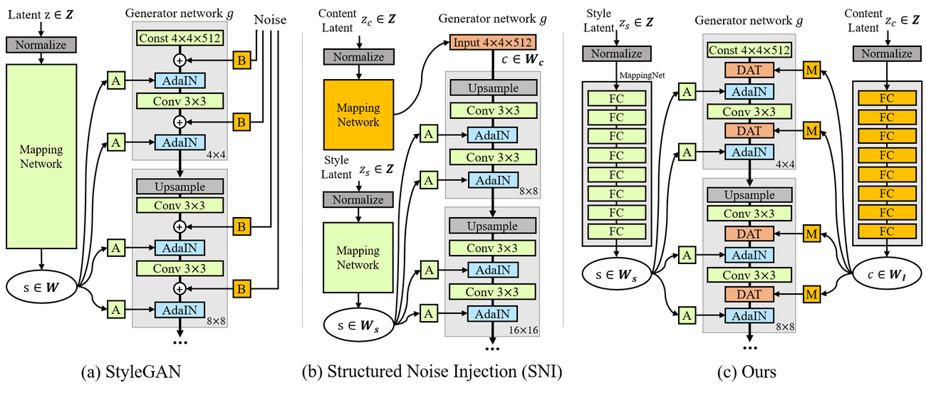
The lecture illustrates 4\times4 pose/geometry, 8\times8 expression, and finer eye/shape changes; these are examples rather than universal layer semantics.
3.6.4 Generator-family comparison
| Model | Spatial/content input | Style mechanism | Distinctive change |
|---|---|---|---|
| StyleGAN | Shared learned constant; per-layer noise | Latent-predicted AdaIN | Per-resolution styles separate from stochastic detail |
| SNI | Local, regional, and global codes build the initial tensor | AdaIN | Structured content enters through the initial spatial tensor |
| Diagonal GAN | Content-predicted diagonal gates at multiple resolutions | AdaIN | Hierarchical spatial/content gating at several resolutions |
The progression in the lecture is therefore constant + stochastic detail -> structured input -> hierarchical spatial gating. The key limitation of ordinary StyleGAN noise is that independent noise mainly changes stochastic local detail rather than providing a stable semantic content control signal (Ye 2026b). SNI introduces structured spatial content but does so asymmetrically at the input; Diagonal GAN makes content control hierarchical, paralleling StyleGAN’s multi-resolution style control.
3.7 Paired and unpaired image translation
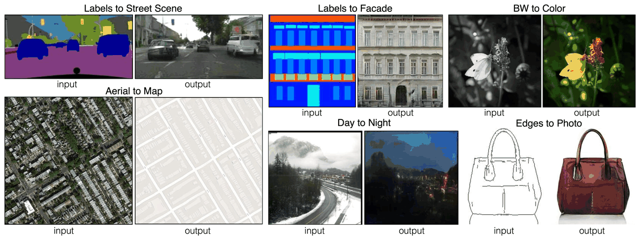
3.7.1 Pix2Pix: realism plus paired reconstruction
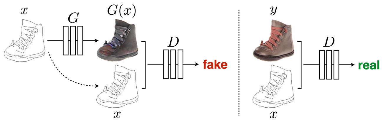
Pix2Pix assumes aligned training pairs (x,y). Its discriminator sees the input together with the proposed output, not the output alone (Isola et al. 2017, sec. 3; Ye 2026a, 114–15):
\begin{aligned} \mathcal{L}_{\mathrm{cGAN}}(G,D)&=\mathbb{E}_{x,y}\log D(x,y) +\mathbb{E}_{x,z}\log(1-D(x,G(x,z))),\\ \mathcal{L}_{\mathrm{pair}}&=\mathbb{E}_{x,y,z}\|y-G(x,z)\|_1,\\ G^*&=\arg\min_G\max_D\left[ \mathcal{L}_{\mathrm{cGAN}}+\textcolor{violet}{\lambda\mathcal{L}_{\mathrm{pair}}}\right]. \end{aligned} \tag{3.14}
The adversarial term tests conditional realism; the paired term anchors the output to the correct target. A U-Net generator preserves aligned structure through skip connections, and a PatchGAN discriminator checks local patches. The paper uses a non-saturating generator update in implementation and finds that explicit input noise tends to be ignored; dropout produces only modest variation.
Advantage: a shared conditional framework for many aligned translation tasks. Limitation: requires paired supervision and does not adequately represent all plausible outputs. It is not unsupervised simply because it uses a GAN.
3.7.2 Why unpaired translation is ill-posed
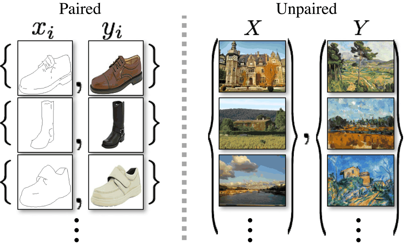
With unpaired collections, we observe marginals p_{\mathcal{X}},p_{\mathcal{Y}}, not the correspondence p(x,y). Matching G_\#p_{\mathcal{X}}=p_{\mathcal{Y}} does not tell us which target belongs to a particular input. For example, two equally likely inputs and two equally likely targets admit both possible bijections with exactly the same marginals. A constraint is necessary, but a constraint need not identify the intended semantics.
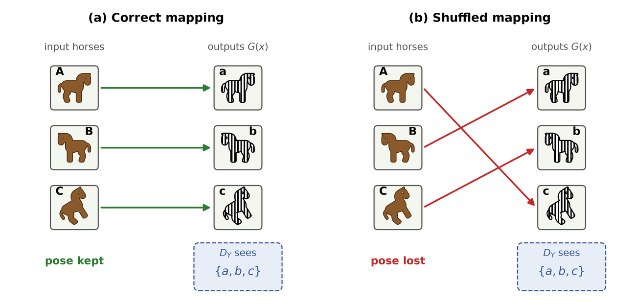
3.7.3 CycleGAN and the role of the cycle
CycleGAN uses G:\mathcal{X}\to\mathcal{Y}, F:\mathcal{Y}\to\mathcal{X}, and two discriminators (Zhu et al. 2017, sec. 3; Ye 2026a, 116–18):
\begin{aligned} \mathcal{L}_{\mathrm{GAN}}(G,D_Y) &=\mathbb{E}_y\log D_Y(y)+\mathbb{E}_x\log(1-D_Y(G(x))),\\ \mathcal{L}_{\mathrm{cyc}} &=\mathbb{E}_x\|F(G(x))-x\|_1+\mathbb{E}_y\|G(F(y))-y\|_1,\\ \min_{G,F}\max_{D_X,D_Y}\quad &\mathcal{L}_{\mathrm{GAN}}(G,D_Y)+\mathcal{L}_{\mathrm{GAN}}(F,D_X) +\textcolor{violet}{\lambda_{\mathrm{cyc}}\mathcal{L}_{\mathrm{cyc}}}. \end{aligned} \tag{3.15}
The reverse adversarial term exchanges x,y and F,G. The cycle compares a reconstructed image to its own input, so it needs no paired target in the other domain. The published implementation uses least-squares adversarial losses; the equation above is the paper’s explanatory log-GAN formulation. An optional identity loss helps preserve appearance when an image is already in the target domain.
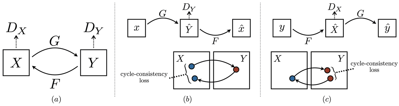
Advantage: learns two-way translation from unpaired data.
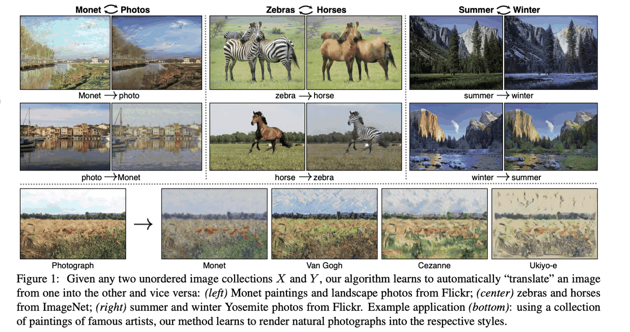
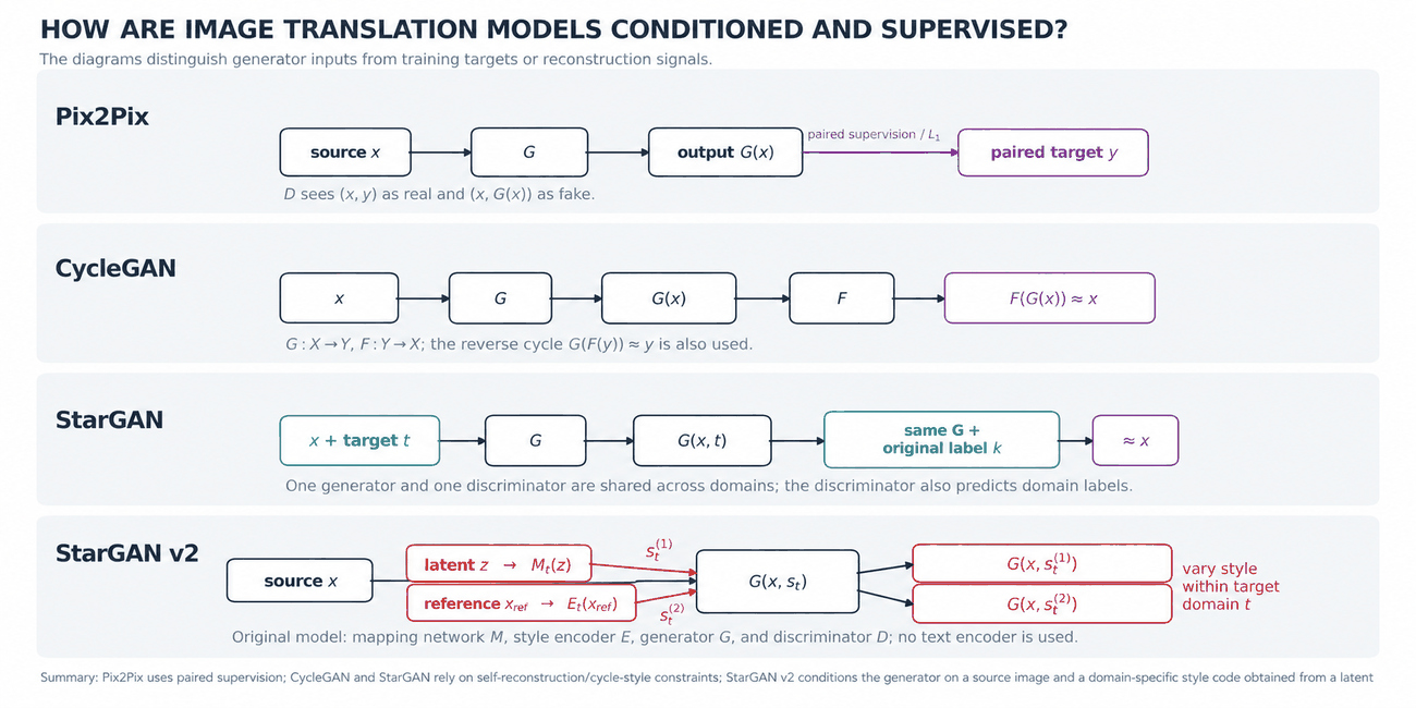
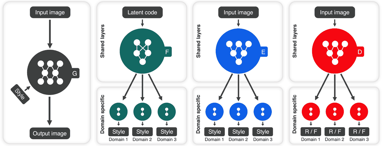
Limitation: cycle consistency does not establish the correct semantic pairing, and optimization is substantially more delicate than in Pix2Pix. The lecture emphasizes the practical reason: CycleGAN jointly trains two generators and two discriminators, so adversarial objectives in both directions interact with the cycle term. In practice the networks are updated alternately rather than by solving a closed-form minimax problem; poorly balanced updates can produce unstable dynamics. This training difficulty was presented in class as an important hands-on lesson, not a minor implementation detail (Ye 2026b). Figure 3.12 contrasts paired supervision, round-trip reconstruction, domain-conditioned reconstruction, and style-code conditioning across the main translation models.
3.8 Multiple domains and multiple inputs
The lecture presents a clear architectural progression. Pairwise CycleGAN/DiscoGAN-style translation scales poorly when every ordered domain pair needs its own mapping. StarGAN replaces those pairwise generators with one shared generator conditioned on a target domain label. StarGAN v2 then replaces the coarse label-only control with a compact, domain-specific style code that can be obtained from either a random latent or a reference image (Ye 2026a, 119–25; 2026b).
3.8.1 Scaling up: DiscoGAN and RadialGAN
For K domains, separate directed pairwise generators require K(K-1) maps: choose one source and one different target. This is a naive pairwise construction, not a universal lower bound. Slide 119 counts K discriminators by sharing one per destination; independently trained CycleGAN pairs instead contain K(K-1) discriminator instances.
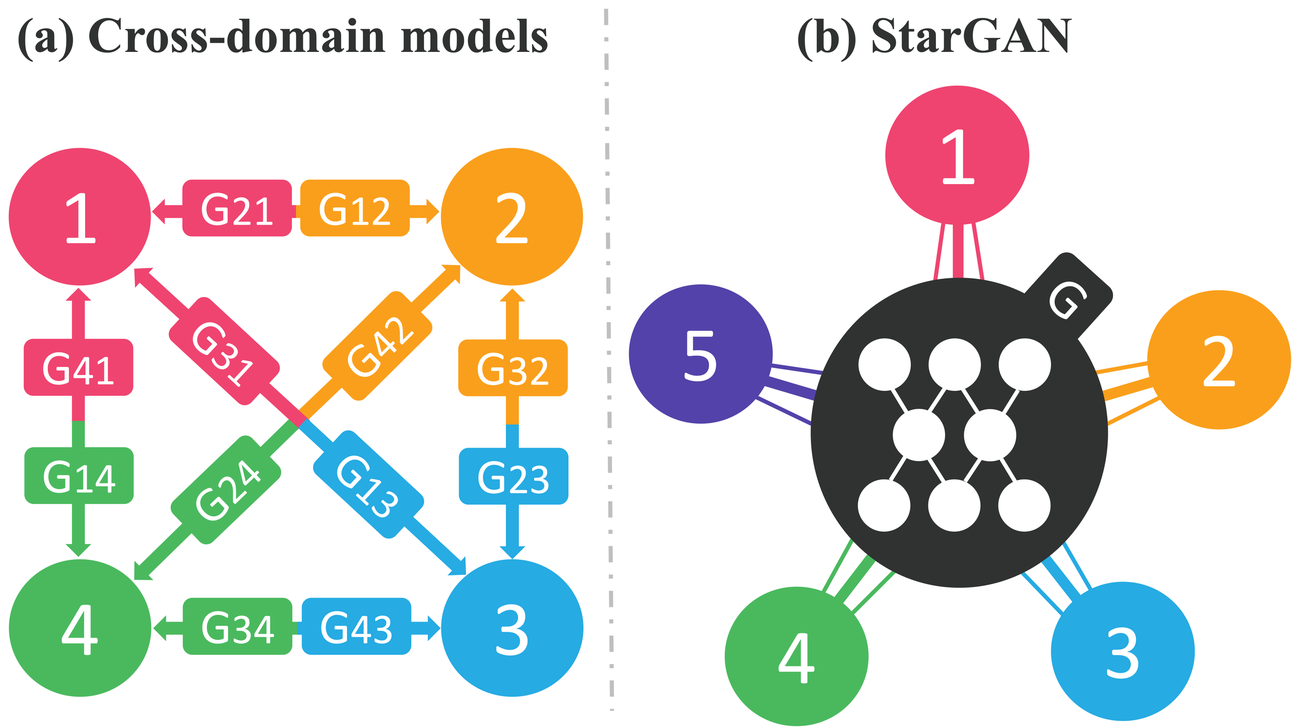
DiscoGAN independently develops bidirectional unpaired translation with adversarial losses and two reconstruction cycles (Kim et al. 2017, sec. 2). In the present notation its generator objective has the structure
\mathcal{L}_G=\mathcal{L}_{\mathrm{adv}}^{X\to Y}+\mathcal{L}_{\mathrm{adv}}^{Y\to X} +\textcolor{violet}{\lambda_X\mathbb{E}_x d(F(G(x)),x) +\lambda_Y\mathbb{E}_y d(G(F(y)),y)}. \tag{3.16}
d is a reconstruction distance; the paper’s illustration uses squared error. Advantage: discovers cross-domain relations without paired targets. Limitation: the basic formulation is two-domain, with the same correspondence ambiguity. It is related to CycleGAN, not necessarily identical in architecture or every loss detail.
RadialGAN routes domains through a shared latent space, with domain-specific encoders E_i and decoders G_j (Yoon et al. 2018, sec. 3):
u_i\ \xrightarrow{E_i}\ z\ \xrightarrow{G_j}\ \hat u_j, \qquad \mathcal{L}_{\mathrm{cyc}}^{i}= \mathbb{E}\|u_i-G_i(E_i(u_i))\|_2+ \mathbb{E}\|z-E_i(G_i(z))\|_2. \tag{3.17}
Here u_i denotes a record including its response in the paper’s continuous-response setting, and z can come from other domains’ encoders. Domain adversarial losses match translated and real records.
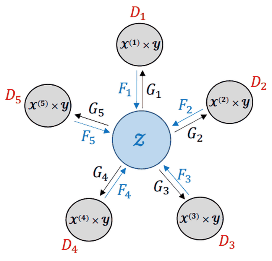
Advantage: O(K) encoder/decoder modules accommodate heterogeneous feature spaces. Limitation: requires a useful shared representation and still uses multiple domain modules. It is originally a predictive-data transfer method, not a many-image fusion model or a single universal generator like StarGAN.
3.8.2 StarGAN: one generator conditioned on a domain label
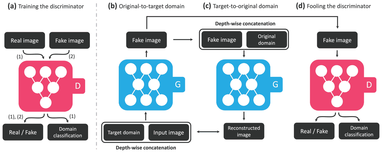
StarGAN spatially replicates a target label t and concatenates it with input x. Its discriminator has a real/fake output and an auxiliary domain classifier (Choi et al. 2018, sec. 3; Ye 2026a, 120–22).
\begin{aligned} \mathcal{L}_{\mathrm{cls}}^{r}&=\mathbb{E}_{x,k}[-\log D_{\mathrm{cls}}(k\mid x)],\\ \mathcal{L}_{\mathrm{cls}}^{f}&=\mathbb{E}_{x,t}[-\log D_{\mathrm{cls}}(t\mid G(x,t))],\\ \mathcal{L}_{\mathrm{rec}}&=\mathbb{E}_{x,k,t}\|x-G(G(x,t),k)\|_1,\\ \mathcal{L}_D&=-\mathcal{V}_{\mathrm{adv}}+\textcolor{teal}{\lambda_{\mathrm{cls}}\mathcal{L}_{\mathrm{cls}}^{r}},\\ \mathcal{L}_G&=\mathcal{V}_{\mathrm{adv}}+\textcolor{teal}{\lambda_{\mathrm{cls}}\mathcal{L}_{\mathrm{cls}}^{f}} +\textcolor{violet}{\lambda_{\mathrm{rec}}\mathcal{L}_{\mathrm{rec}}}. \end{aligned} \tag{3.18}
\mathcal{V}_{\mathrm{adv}} is the paper’s log-GAN value in its explanatory formulation; its experiments replace this with WGAN-GP. Classification on real images trains D; classification on generated images trains G. The same G is used twice for reconstruction. A dataset mask can indicate which labels are known when training jointly on datasets with different annotation sets.
Advantage: shares parameters across domains instead of training every pair separately. Limitation: the original deterministic mapping offers one output for fixed (x,t) and needs domain labels. Label concatenation does not provide within-domain style diversity or fuse several source images.
3.8.3 StarGAN v2: diverse, domain-specific style codes
StarGAN v2 replaces the fixed label input to G with a style code injected through AdaIN. A mapping network M_t(z) supplies latent-guided styles; a style encoder E_t(x_{\mathrm{ref}}) supplies reference-guided styles. M, E, and D have domain-specific output heads, while G is shared (Choi et al. 2020, sec. 2; Ye 2026a, 123–25).
\textcolor{red}{s_t}=M_t(z)\ \text{or}\ E_t(x_{\mathrm{ref}}),\qquad \hat x=G(x,\textcolor{red}{s_t}),\qquad s_k=E_k(x). \tag{3.19}
Its key training terms, for s_t^i=M_t(z_i), are
\begin{aligned} \mathcal{V}_{\mathrm{adv}}&=\mathbb{E}_{x,k}\log D_k(x) +\mathbb{E}_{x,t,z}\log(1-D_t(G(x,s_t))),\\ \mathcal{L}_{\mathrm{sty}}&=\mathbb{E}\|s_t-E_t(G(x,s_t))\|_1,\\ \mathcal{L}_{\mathrm{ds}}&=\mathbb{E}\|G(x,s_t^1)-G(x,s_t^2)\|_1,\\ \mathcal{L}_{\mathrm{cyc}}&=\mathbb{E}\|x-G(G(x,s_t),s_k)\|_1,\\ \min_{G,M,E}\max_D\quad &\mathcal{V}_{\mathrm{adv}} +\textcolor{red}{\lambda_{\mathrm{sty}}\mathcal{L}_{\mathrm{sty}}} -\textcolor{orange}{\lambda_{\mathrm{ds}}\mathcal{L}_{\mathrm{ds}}} +\textcolor{violet}{\lambda_{\mathrm{cyc}}\mathcal{L}_{\mathrm{cyc}}}. \end{aligned} \tag{3.20}
Style reconstruction prevents ignoring the style input; the minus sign rewards different outputs; the cycle promotes source preservation. Unlike Diagonal GAN’s thresholded diversity loss, \mathcal{L}_{\mathrm{ds}} here is a distance reward. Recovering s_t from a generated image does not force two unrelated latent- and reference-derived styles to be equal.
Advantage: latent and reference control with multiple outputs per target domain. Limitation: multiple objectives must balance diversity and preservation, and trained domains still need labels. The original model has neither a text encoder nor text cross-attention; the transcript’s diffusion/text comparison is an analogy.
3.8.4 Comparison at a glance
| Model | Input information | Added constraint or control | Main unresolved issue |
|---|---|---|---|
| Pix2Pix | Paired (x,y) | Paired L_1 reconstruction + conditional discriminator | Requires aligned pairs; limited multimodality |
| CycleGAN / DiscoGAN | Unpaired two-domain collections | Two adversarial directions + reconstruction cycle | Training stability and semantic ambiguity |
| RadialGAN | Heterogeneous domains | Shared latent + domain-specific encoders/decoders | Quality of the shared representation |
| StarGAN | One image + target domain label | Domain classification + shared-generator reconstruction | One output for fixed (x,t) |
| StarGAN v2 | One image + latent/reference style | Style recovery + diversity + reconstruction | Diversity/preservation trade-off |
The main change from StarGAN to StarGAN v2 is not simply “more domains.” StarGAN says which target domain is desired; StarGAN v2 additionally supplies which style inside that domain. This makes latent-guided and reference-guided multimodal outputs possible while keeping a single shared image generator.
Training versus inference. Discriminator updates treat generated images as detached samples. Generator updates propagate gradients through the discriminator while holding its parameters fixed; the cycle also backpropagates through the participating generators. Inference uses the trained generator and its required conditioning modules, not the discriminator. The distinction between a minimax value and the loss minimized by each optimizer is therefore important.
3.9 Worked examples and reproducibility
3.9.1 AdaIN with actual numbers
Take one content channel u=(1,3)^\top and reference channel v=(2,6)^\top. Their means are 2,4 and their population standard deviations are 1,2. Equation 3.3 gives
\operatorname{AdaIN}(u,v)=2(u-2\mathbf1)+4\mathbf1=(2,6)^\top.
The transformed channel has the target mean and variance. It does not follow that the output image equals the style image: only these feature statistics were constrained.
3.9.2 Matching marginals does not match correlations
Let a=\sqrt2 and choose centered two-channel feature matrices
X=\begin{bmatrix}a&0\\-a&0\\0&a\\0&-a\end{bmatrix},\qquad S=\begin{bmatrix}a&a/2\\-a&-a/2\\0&\sqrt{3/2}\\0&-\sqrt{3/2}\end{bmatrix}.
Then \Sigma_X=I_2 and \Sigma_S=\begin{bmatrix}1&1/2\\1/2&1\end{bmatrix}. Both channels already have mean zero and standard deviation one. AdaIN therefore leaves X unchanged and misses the target correlation. WCT multiplies X by \Sigma_S^{1/2} and obtains the requested covariance. This is a finite-dimensional counterexample to interpreting AdaIN as full covariance matching.
The following self-contained NumPy example verifies these claims; it is a mathematical check, not a GAN training experiment.
import numpy as np

def cov(x):
    xc = x - x.mean(axis=0, keepdims=True)
    return xc.T @ xc / x.shape[0]

def spd_power(a, power):
    vals, vecs = np.linalg.eigh(a)
    if np.any(vals <= 0):
        raise ValueError("This example requires positive-definite covariance.")
    return (vecs * vals**power) @ vecs.T

a = np.sqrt(2.0)
x = np.array([[a, 0], [-a, 0], [0, a], [0, -a]])
s = np.array([[a, a/2], [-a, -a/2],
              [0, np.sqrt(1.5)], [0, -np.sqrt(1.5)]])
adain = (x - x.mean(0)) / x.std(0) * s.std(0) + s.mean(0)
wct = ((x - x.mean(0)) @ spd_power(cov(x), -0.5)
       @ spd_power(cov(s), 0.5) + s.mean(0))
assert np.allclose(cov(adain), np.eye(2))
assert np.allclose(cov(wct), cov(s))
print("AdaIN covariance:\n", np.round(cov(adain), 6))
print("WCT covariance:\n", np.round(cov(wct), 6))
3.10 Connections and further reading
The lecture’s central connection is between where a representation is transformed and what a translation objective constrains. Normalization/AdaIN act mainly on the channel axis, while spatial attention acts on the position axis; the unified Y=AXT+B view makes this distinction explicit. StyleGAN, SNI, and Diagonal GAN then turn these transforms into architectural control signals at different resolutions. Pix2Pix, CycleGAN, StarGAN, and StarGAN v2 add progressively different kinds of supervision: paired targets, round-trip reconstruction, domain labels, and domain-specific style codes.
The main lecture should therefore be read as one progression rather than a list of GAN variants: statistics -> axis-wise feature transforms -> controllable synthesis -> translation constraints -> scalable multi-domain conditioning. The brief paper extensions above are useful related reading, but they are intentionally separated from the pp. 78–125/script narrative.
3.11 Advanced topics
The chapter above follows the lecture and its Part 1 --- GAN pages. This section develops the points the lecture named and left, and the derivations the main text states without giving. Each subsection is self-contained and none is needed to follow the main line.
3.11.1 Gram matrices, and why AdaIN is their diagonal case
Before AdaIN, neural style transfer represented style by correlations of fixed encoder features. With \Phi_\ell(I)\in\mathbb{R}^{N_\ell\times C_\ell} and \Gamma_\ell(I)=\Phi_\ell(I)^\top\Phi_\ell(I), a representative objective is (Gatys et al. 2016)
\mathcal{L}_{\mathrm{style}}= \sum_\ell a_\ell\|\Gamma_\ell(I_o)-\Gamma_\ell(I_s)\|_F^2, \qquad \mathcal{L}_{\mathrm{content}}=\|\Phi_{\ell_c}(I_o)-\Phi_{\ell_c}(I_c)\|_F^2. \tag{3.21}
A Gram matrix is unchanged by a permutation of spatial positions, so it captures channel co-occurrence statistics more readily than layout. Advantage: rich multi-layer appearance matching. Limitation: the original method optimizes each output image iteratively and does not guarantee content preservation. AdaIN is a feed-forward statistic-matching alternative, not an exact solver of the Gram objective.
That is the statement. Why a Gram matrix is a representation of style at all, and how it connects to the AdaIN the chapter has already used, is the part worth spelling out.
Write \Phi_\ell(I) \in \mathbb{R}^{N_\ell \times C_\ell} for the features of a frozen VGG layer, rows indexed by position and columns by channel. Then \Gamma_\ell = \Phi_\ell^\top \Phi_\ell has entries \Gamma_{cc'} = \sum_n \Phi_{nc}\Phi_{nc'}: an uncentred second-order statistic of the channels, summed over positions. Permuting the rows of \Phi_\ell leaves \Gamma_\ell unchanged, which is the sense in which it discards layout; what survives is which channels fire together, and for a convolutional encoder a channel is a texture detector, so co-occurrence of channels is texture. That is the whole argument, and it also bounds what the representation can do: anything that depends on where the texture is placed is invisible to it.
Which layer carries what is an empirical choice, and the usual one is that content is read off a single deep layer — relu4_2 in Gatys et al. — where the representation is coarse enough to be insensitive to appearance, while style is read off several layers at once, relu1_1 through relu5_1, because texture lives at every scale. The weights a_\ell in Equation 3.21 balance them, and each layer’s term is usually divided by 4 N_\ell^2 C_\ell^2 so that layers of different size contribute comparably.
The cost of the original method is the reason AdaIN exists. Gatys et al. produce each output by optimising the image: start from noise or from the content image and run L-BFGS on \mathcal{L}_{\mathrm{content}} + \mathcal{L}_{\mathrm{style}} for hundreds of iterations, each one a forward and backward pass through VGG. Every new content-style pair pays this again.
Now the link. Take the diagonal of the Gram matrix and nothing else. Matching \Gamma_{cc} for every c matches each channel’s second moment, and matching the feature means as well makes it each channel’s mean and variance — which is exactly what Equation 3.3 does, in closed form, in one pass. AdaIN is therefore the diagonal special case of Gram matching, computed rather than optimised, and WCT of Equation 3.6 is the step that puts the off-diagonal entries back. The three sit on one axis: diagonal second moments (AdaIN), full covariance (WCT), full uncentred Gram across several layers (Gatys).
3.11.2 The feed-forward form of style transfer
Equation 3.3 is a transform, not a method: something has to turn the transformed features back into an image. Huang and Belongie train a decoder g against a frozen VGG encoder f, and the two losses are worth writing out because the first is not the obvious one.
With t = \operatorname{AdaIN}(f(c), f(s)) the target features and T = g(t) the output image,
\mathcal{L}_c = \|f(T) - t\|_2 , \qquad \mathcal{L}_s = \sum_{\ell} \Big( \|\mu(\phi_\ell(T)) - \mu(\phi_\ell(s))\|_2 + \|\sigma(\phi_\ell(T)) - \sigma(\phi_\ell(s))\|_2 \Big) , \tag{3.22}
minimising \mathcal{L}_c + \lambda \mathcal{L}_s over the decoder alone. The content loss is the distance to the AdaIN output t, not to f(c): the decoder is asked to reproduce the transformed features, not the original ones, which is what lets a single decoder serve every style. The style loss matches means and standard deviations across several VGG layers — the diagonal statistics of Section 3.11.1, again — rather than Gram matrices, and Huang and Belongie report the two give comparable results at lower cost.
Because the transform is explicit, two knobs come for free at test time and need no retraining. Interpolating t towards f(c),
T_\alpha = g\big( (1-\alpha) f(c) + \alpha \operatorname{AdaIN}(f(c), f(s)) \big) , \tag{3.23}
trades content against style continuously, with \alpha = 0 reconstructing the content image. Interpolating between several styles’ AdaIN targets mixes styles. Neither is available to a decoder trained per style.
3.11.3 Why the W space disentangles better than Z
The chapter answers this in one sentence — the mapping can reshape the prior — and the standard account is worth the extra paragraph, because it explains what goes wrong in \mathcal{Z} rather than only what is better in \mathcal{W}.
The prior on \mathcal{Z} is fixed, z \sim \mathcal{N}(0,I), and the generator must push it onto the data distribution. Suppose some combination of attributes is absent from the training data — long hair together with a masculine face, in the paper’s example. The generator cannot map any region of \mathcal{Z} to that combination, so the map from \mathcal{Z} to attributes has to curve around the missing region. A curved map does not have axes: moving along a straight line in \mathcal{Z} changes several attributes at once, which is entanglement, and it is forced by the shape of the data together with the fixed shape of the prior.
\mathcal{W} is under no distributional constraint at all. Nothing requires w = f(z) to be Gaussian, or to have any particular density, so the mapping network can absorb the warping: f takes the curvature and the synthesis network sees a space in which the factors can be closer to axis-aligned.
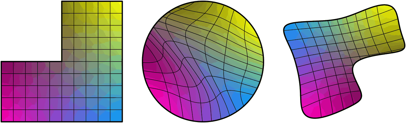
The claim is that the warping has to happen somewhere and it is better done in a learned space than forced into the generator.
Two measurements support it, and both deserve their definitions rather than their names. Perceptual path length samples two latents, interpolates a short step \epsilon between them, and measures the perceptual distance between the two images, averaged and normalised by \epsilon^2:
\mathrm{PPL} = \mathbb{E}\left[ \tfrac{1}{\epsilon^{2}}\, d_{\mathrm{VGG}}\big( G(\mathrm{lerp}(w_1,w_2;t)),\, G(\mathrm{lerp}(w_1,w_2;t+\epsilon)) \big) \right] . \tag{3.24}
A small value says the image changes at a steady rate along the path — that the latent space is not curved — and it is the operational reading of “less entangled”. Linear separability is the complementary test: train an auxiliary classifier on a binary attribute, then ask how well a linear hyperplane in latent space separates the two classes, reported as a conditional entropy. Both come out better for \mathcal{W} than for \mathcal{Z}.
Two mechanisms in the paper follow directly. Truncation samples w and pulls it towards the mean, w' = \bar{w} + \psi(w - \bar{w}) with \psi < 1, trading variety for quality; it is done in \mathcal{W} precisely because distances there are the perceptually meaningful ones. Style mixing draws two codes and uses one before a randomly chosen layer and the other after, during training, which stops the network from assuming that adjacent layers’ styles are correlated — the regulariser that makes the per-resolution control of Equation 3.10 actually hold.
3.11.4 StyleGAN’s noise, and what it is for
The chapter defines n_\ell correctly and asserts its role. The evidence is an ablation, and it is worth stating because it is what separates stochastic variation from style as the chapter uses the words.
The attributes the noise controls are the ones a viewer cannot name as different: the exact placement of hair strands, freckles, skin pores, the precise outline of the background. Resampling the noise with w held fixed changes all of these and changes nothing a human would call the person’s appearance. Removing the noise entirely does not give a cleaner image; it gives a flat, painterly one, because the generator has no source of variation for detail that ought to differ between samples and produces a featureless average instead.
The scale experiment is what makes it an argument about architecture rather than about texture. Noise fed only to the coarse layers moves large features — the overall curl of the hair; noise fed only to the fine layers moves only the finest detail. So the noise inherits the resolution of the layer it enters, exactly as the styles do in Equation 3.10, and the two channels are independent: w sets what the image is, n sets the arbitrary part of how it is realised.
3.11.5 StyleGAN2: demodulation and path-length regularization
StyleGAN2 removes explicit instance normalization from the synthesis path and modulates/demodulates convolution weights (Karras et al. 2020). If s_i is a style scale for input channel i,
w'_{ijk}=\textcolor{red}{s_i}w_{ijk},\qquad w''_{ijk}=\frac{w'_{ijk}} {\sqrt{\sum_{i',k'}(w'_{i'jk'})^2+\epsilon}}. \tag{3.25}
Demodulation controls the expected output scale without normalizing each observed feature map, addressing the characteristic droplet artifacts associated with the original normalization design. StyleGAN2 also uses path-length regularization,
\mathcal{L}_{\mathrm{pl}}= \mathbb{E}_{w,r}\left(\|J_g(w)^\top r\|_2-a\right)^2, \tag{3.26}
which encourages a more uniform sensitivity of the generated image to changes in w. Advantage: cleaner style modulation and fewer normalization artifacts. Limitation: these regularizers improve conditioning but do not guarantee semantic disentanglement.
Three points make the equations above an argument rather than a recipe.
Where the droplet comes from. Instance normalization standardises each feature map after the convolution, which means a generator can put a very large value in one spatial location and have the normalisation scale everything else down around it. The strong local signal survives, because it is what sets the scale; the rest of the map is suppressed. That is the droplet — a blob-shaped artefact that appears in the feature maps from 64\times64 onwards and, once the network depends on it, in the output. Removing normalisation from the forward path removes the mechanism.
Why dividing by that particular norm works. Suppose the inputs to the convolution are independent with unit variance. After modulation the output j has variance \sum_{i,k}(w'_{ijk})^{2}, so dividing the weights by \sqrt{\sum_{i',k'}(w'_{i'jk'})^{2}} restores unit output variance. The essential difference from instance normalization is the object being normalised: this acts on the weights, using the expected statistics under an assumption about the input, and not on the observed feature map. The generator therefore has no observed quantity to game, which is why the droplet does not come back.
The regulariser and its metric. In Equation 3.26 the constant a is not a hyperparameter but a running exponential average of the observed \|J_g(w)^\top r\|_2, so the term penalises deviation from the network’s own current average sensitivity rather than from a chosen value. Its cost is a Jacobian-vector product, so it is applied lazily, once every 16 minibatches, with the step size scaled accordingly. And it is the same quantity the perceptual path length of Equation 3.24 measures: StyleGAN2 regularises the metric that StyleGAN introduced to diagnose entanglement, which is why the two move together. StyleGAN2 also drops progressive growing, whose phase-in of new resolutions left a preference for fixed detail locations, in favour of skip and residual connections that train at full resolution throughout.
3.11.6 The solution set of unpaired translation
The chapter’s two-point example shows that two bijections match the marginals. The situation is worse than “two”, and saying how much worse is what justifies everything that follows it.
Let G satisfy G_{\#}p_{\mathcal{X}} = p_{\mathcal{Y}} and let \tau be any measure-preserving automorphism of (\mathcal{Y}, p_{\mathcal{Y}}), that is, any map with \tau_{\#}p_{\mathcal{Y}} = p_{\mathcal{Y}}. Then
(\tau \circ G)_{\#} p_{\mathcal{X}} = \tau_{\#}\big( G_{\#} p_{\mathcal{X}} \big) = \tau_{\#} p_{\mathcal{Y}} = p_{\mathcal{Y}} , \tag{3.27}
so \tau \circ G is just as valid. For a continuous p_{\mathcal{Y}} the group of such \tau is infinite-dimensional, so the adversarial objective alone picks out nothing: its solution set is an orbit, not a point.
Cycle consistency shrinks the set but does not collapse it. Requiring F \circ G \approx \mathrm{id} forces G to be approximately invertible, which removes the \tau that destroy information; it does not remove the ones that are themselves invertible, and a swap of two equally likely modes is invertible. So what actually identifies the intended map is neither term. It is the architecture: a residual convolutional generator with a receptive field much smaller than the image, trained from an identity-like initialisation, finds small, local, low-frequency changes far more easily than a global rearrangement. The inductive bias is doing the identification, which is why the failures in Section 3.11.7 are the ones they are.
3.11.7 How cycle consistency fails
Two failures are named in the chapter. Both are worth developing, because each is a consequence of the objective rather than an accident of training.
Steganography. Chu et al. showed that a CycleGAN trained on aerial photographs and maps reconstructs features of the source that are not visible in the intermediate image at all: a building absent from the generated map reappears in the reconstruction. The generator has learned to encode the source in a low-amplitude, high-frequency signal that the map-domain discriminator cannot see and the reverse generator can read. The cycle loss is then near zero while the intermediate image is semantically wrong — the objective is satisfied and the task is not.
The mechanism follows from what is penalised. The cycle term constrains the composition F \circ G, not G alone, so any information channel that survives the round trip is rewarded, whether or not it is part of the visible translation. Adding noise to the intermediate image, or otherwise destroying the high-frequency channel, degrades the reconstruction sharply — which is the test that distinguishes hidden information from honest translation.
Geometry. The original CycleGAN paper reports the limitation plainly: tasks requiring shape change fail while tasks requiring texture change succeed. Apple to orange keeps the apple’s outline and repaints it; horse to zebra paints stripes on the horse, and on a rider as well if one is present, because nothing in the objective knows that a rider is not a horse; dog to cat produces minimal change. The reason is the same inductive bias as in Section 3.11.6, read the other way: a residual convolutional generator is well suited to recolouring a pixel from its neighbourhood and badly suited to moving content across the image, and a PatchGAN discriminator judges local patches, so it scores texture and is largely blind to global shape. Neither network is asked for geometry and neither provides it.
3.11.8 OT-driven CycleGAN and CycleGAN failure modes
A related optimal-transport formulation derives CycleGAN rather than modifying it (Sim et al. 2020). It is worth following the direction of that derivation, because it answers the question the lecture leaves open — where the cycle term comes from — and the answer is the opposite of what the shape of the objective suggests.
Start from a Kantorovich problem between the two domains, with a joint transport cost that charges a pair (x,y) for the round trip under the two maps R:\mathcal{Y}\to\mathcal{X} and H:\mathcal{X}\to\mathcal{Y},
d\big((x,y)\big)=\|x-R(y)\|+\|y-H(x)\|. \tag{3.28}
Minimising \int d \, d\pi over couplings \pi of p_{\mathcal{X}} and p_{\mathcal{Y}} is the primal problem, and its objective is the cycle/data-consistency term: Equation 3.28 is what \mathcal{L}_{\mathrm{cyc}} measures. The marginal constraints are then relaxed by Kantorovich duality, and it is the dual of those constraints that produces two Wasserstein-1 terms, each realised by a 1-Lipschitz critic. Collecting the two,
\min_{R,H} \textcolor{violet}{\lambda\mathcal{L}_{\mathrm{cyc}}(R,H)} +W_1(p_{\mathcal X},R_\#p_{\mathcal Y})+ W_1(p_{\mathcal Y},H_\#p_{\mathcal X}). \tag{3.29}
So the reading to carry away is not “W_1 matching, plus a cycle penalty of unexplained origin”. It is: the cycle term is the transport cost, and the adversarial terms are the penalties that enforce the marginals. The weight \lambda is the exchange rate between the two, and taking \lambda large is what recovers the hard marginal constraints of the original Kantorovich problem. The critics are 1-Lipschitz because that is what the dual asks for, not because a Lipschitz constraint was found to stabilise training.
This remains a surrogate training objective once the ideal critic class is replaced by neural networks, so the equality between theory and implementation should not be overstated.
Cycle consistency also has important failure modes. First, it does not identify the intended semantic pairing: two domains with two equally likely elements admit a swapped bijection with perfect marginal matching and zero cycle error. Second, a network can hide source information in visually weak high-frequency signals and use it to reconstruct the input, producing a small cycle loss without meaningful visible preservation (Chu et al. 2017). Large geometric changes were also reported as difficult in the original CycleGAN study (Zhu et al. 2017). Thus realistic marginals plus a small cycle loss are not a certificate of correct correspondence.
3.11.9 StarGAN’s mask vector
The chapter mentions the mask in a clause. It is what lets one generator train on two datasets whose label sets do not overlap — CelebA with facial attributes, RaFD with expressions — and the encoding is simple enough to give in full.
The label fed to the generator is a concatenation \tilde{c} = [c_1, \dots, c_n, m], where c_i is the label vector for dataset i and m is a one-hot mask naming which dataset the current example came from. The entries of every c_i but the active one are set to zero and are to be ignored. The generator learns to read m and attend to the corresponding block, so a CelebA example carries expression bits that are zero and uninformative rather than zero and meaningful.
The discriminator’s classification head is split to match: it predicts labels for both datasets, and the classification loss for an example is computed only over the head belonging to its own dataset. Without the mask the zeros would be indistinguishable from genuine negative labels, and the generator would learn that every CelebA face has a neutral expression.
3.11.10 CollaGAN: many inputs, one output
CollaGAN considers a different data regime from StarGAN: several corresponding domain observations of the same subject are available and one target domain is missing (Lee et al. 2019). With target domain t withheld,
\hat x_t=G(\textcolor{blue}{\{x_j:j\ne t\}},t),\qquad \mathcal{L}_{\mathrm{mcyc}}= \mathbb{E}_t\sum_{j\ne t}\|x_j-\tilde x_{j\mid t}\|_1. \tag{3.30}
The multiple-cycle construction reconstructs each available input after inserting the predicted missing image. Advantage: it can fuse complementary observations from several domains. Limitation: it requires corresponding multi-domain input sets, so it solves a different problem from single-input unpaired translation.
That is the summary. The setting deserves more, because it is the one where this lab’s own work sits and because the objective is not a relabelling of StarGAN’s.
The problem is imputation with several co-registered observations: N MR contrasts of the same slice, one of which is missing. A single-input translation model must pick one available contrast and discard the rest. CollaGAN takes all of them, so the generator is a map G(\{x_i\}_{i \ne t}, t) \mapsto \hat{x}_t, from every available input plus a target index to the missing one.
Cycle consistency has to be rebuilt for that signature, and the two-step form is the point of the paper. Having produced \hat{x}_t, put it back into the input set in place of the real x_t and ask for some other contrast j:
\tilde{x}_{j \mid t} = G\big( \{\hat{x}_t\} \cup \{x_i : i \ne t, j\},\; j \big) , \qquad \mathcal{L}_{\mathrm{mcc}} = \sum_{j \ne t} \big\| x_j - \tilde{x}_{j \mid t} \big\|_1 . \tag{3.31}
A single round trip would only check that \hat{x}_t is invertible back to where it came from; this multiple cycle checks that it is consistent with every other contrast at once, which is what a wrong but plausible \hat{x}_t fails. The discriminator carries a classification head over contrasts, as in Equation 3.18, so the output must also be recognisable as contrast t. For MR synthesis the reconstruction term is supplemented by a structural-similarity term, since L_1 alone tolerates the loss of fine structure that matters clinically.
The reason the collaborative version wins is worth stating plainly: the contrasts are different measurements of the same anatomy, so what is missing from one is usually present in another. A model that reads only one of them throws away exactly the redundancy the problem provides.
Based on the scribe note of Jeongchan Kim, with material from Daegyu Sung, Seungwan Kang and Chaeyoung Oh; edited by Jong Chul Ye.