5 Self-supervised Denoising
5.1 Overview
The previous lectures built generative models that learn a data distribution directly: GANs through an adversarial game, VAEs through the ELBO, and normalizing flows through an exact change of variables. This lecture takes a step sideways to a problem that looks much more modest, image denoising, and asks a question that turns out to lead straight into the diffusion half of the course: can a network learn to remove noise when it has never seen a clean image?
We first place denoising inside the general inverse problem and recall the classical answer (regularized least squares and BM3D) and the first deep answer (supervised training, DnCNN). Supervised training needs clean targets, which are often physically impossible to obtain. Three families of methods avoid them: Noise2Noise trains on pairs of independent noisy copies; Noise2Self and Noise2Void train on a single noisy copy with a blind-spot network; SURE trains on a single noisy copy with a divergence penalty. These look like unrelated heuristics. The second half of the lecture shows that they are not: Tweedie’s formula says that the Bayes-optimal denoiser is determined by the score \nabla_y \log p(y) of the noisy data. For Gaussian noise all three methods can then be understood through the relation between the score and the conditional mean that each of them targets. Noise2Score makes this explicit, estimates the score once, and then applies the Tweedie formula that matches the noise model (Gaussian, Poisson, Gamma, and others).
The same decomposition — learn a score during training, use it through Tweedie’s formula at inference — is the core of diffusion models, which is why this lecture sits between the VAE/flow lectures and DDPM. After reading this chapter you should be able to prove why Noise2Noise and Noise2Self do not collapse, derive SURE from Stein’s lemma, derive Tweedie’s formula for any exponential-family noise model, and explain why “denoising is score estimation”.
5.2 Notation
We follow the notation of the slides and of Geometry of Deep Learning (Ye 2022).
| Symbol | Meaning |
|---|---|
| x \in \mathbb{R}^n | the unknown clean image, flattened to n pixels |
| y \in \mathbb{R}^n | the noisy measurement |
| w | additive noise; in the Gaussian case w \sim \mathcal{N}(0, \sigma^2 I) |
| \mathcal{A} | forward (imaging) operator of a general inverse problem |
| F_\Theta | denoising network with parameters \Theta; \hat{x} = F_{\Theta^*}(y) |
| \mathcal{R}(y; \Theta), R_\Theta | network in residual form: the DnCNN noise predictor, or a score network |
| P_Y | distribution of the noisy data; p(y) its density |
| l(y) = \log p(y) | log-density of the noisy data |
| l'(y) = \nabla_y \log p(y) | the score function of the noisy data |
| \eta, T(y), p_0(y), \varphi(\eta) | natural parameter, sufficient statistic, base measure and log-partition function of an exponential family |
| l_0(y) = \log p_0(y) | log of the base measure; l_0'(y) its derivative |
| \lambda(y) = \log \frac{p(y)}{p_0(y)} | log-ratio appearing in the posterior of \eta |
| \operatorname{div}_y F | divergence \sum_i \partial F_i / \partial y_i, the trace of the Jacobian |
| \sigma_a | the artificial noise level added in a denoising autoencoder |
References of the form “slide 12” point to the 38-page lecture deck Self-supervised Image Denoising (Ye 2026), so that each section can be checked against the lecture. Norms are Euclidean. The slides write the score both as l'(y) and \ell'(y); we use l'(y) throughout. A prime on a function of a vector y means its gradient. Expectations without a subscript are over everything that is random in the expression.
5.3 Denoising as an inverse problem
5.3.1 The forward model and ill-posedness
An imaging system (slide 3) — a microscope, a telescope, a CT scanner — maps an unknown object x to a measurement through a forward operator \mathcal{A}, and the measurement is corrupted by noise (Figure 5.1):
y = \mathcal{A}(x) + w . \tag{5.1}
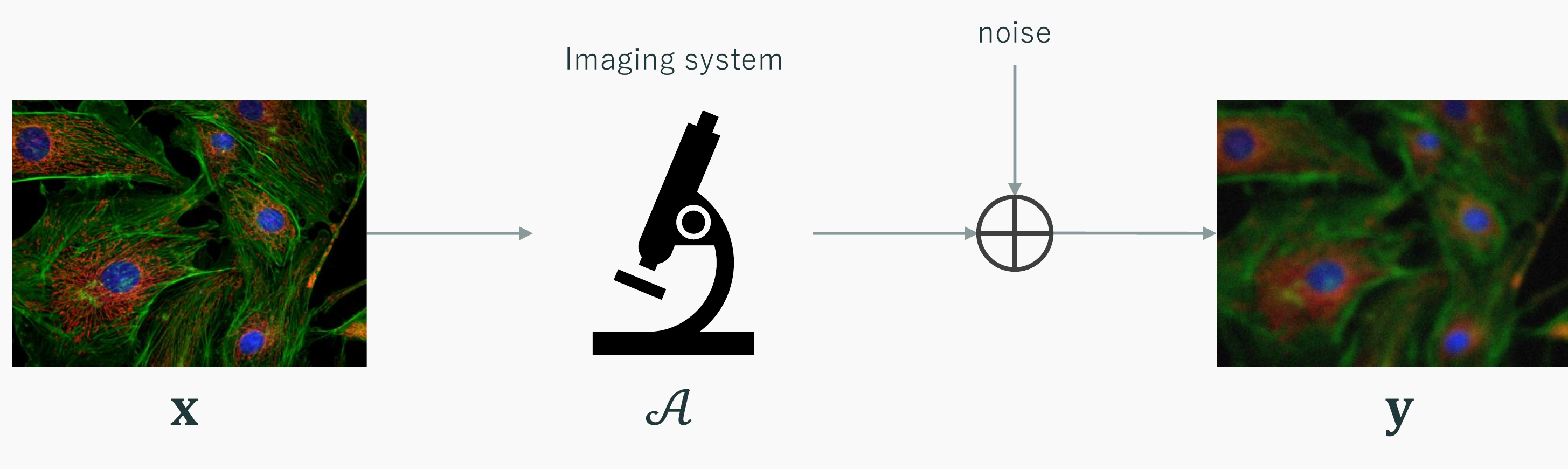
In the fluorescence microscopy example of the lecture, \mathcal{A} is convolution with the optical point-spread function, which blurs everything below the diffraction limit. Recovering x from y is an inverse problem, and it is typically ill-posed: many different x produce the same blurred and noisy y, so the data alone do not determine the answer. The question is not “what is the solution” but “which of the infinitely many candidates is the best one, and in what sense”.
Denoising is the special case \mathcal{A} = I:
y = x + w . \tag{5.2}
It is ill-posed for the same reason — every x is consistent with y for some noise realization — and it is the building block for the general case, because most modern solvers for Equation 5.1 alternate a data-consistency step with a denoising step.
5.3.2 Classical regularization
The classical remedy (slide 4) restricts the solution space with prior knowledge:
\min_x \; \frac{1}{2}\|y - \mathcal{A}(x)\|_2^2 + \lambda R(x) . \tag{5.3}
The first term is the data fidelity; the second is a regularizer that is small for plausible images. Common choices in the lecture were sparsity (R(x) = \|x\|_1, natural in fluorescence imaging where most pixels are dark), total variation (R(x) = \sum_i \|(\nabla x)_i\|, which favours piecewise-constant images), and regularization by denoising (RED), where an off-the-shelf denoiser D defines R(x) = \frac{1}{2} x^\top (x - D(x)) (Romano et al. 2017).
It is worth seeing that Equation 5.3 is a Bayesian estimate in disguise, because the second half of this lecture is entirely Bayesian. With Gaussian noise w \sim \mathcal{N}(0, \sigma^2 I) the likelihood is p(y \mid x) \propto \exp(-\|y - \mathcal{A}(x)\|^2 / 2\sigma^2). If the prior is p(x) \propto \exp(-\lambda R(x)/\sigma^2), Bayes’ rule gives
-\log p(x \mid y) = \frac{1}{2\sigma^2}\|y - \mathcal{A}(x)\|^2 + \frac{\lambda}{\sigma^2} R(x) + \text{const},
so minimizing Equation 5.3 is the same as maximizing the posterior (MAP estimation). The regularizer is, up to the factor \lambda/\sigma^2 and an additive constant, a negative log-prior. Choosing R by hand is choosing the prior by hand; learning-based methods instead learn it from data. The score-based view at the end of this chapter is related but not identical: it learns the score \nabla_y \log p(y) of the noisy data, which differs from the gradient of the clean log-prior \log p(x) unless the noise vanishes.
5.3.3 BM3D: collaborative filtering of similar patches
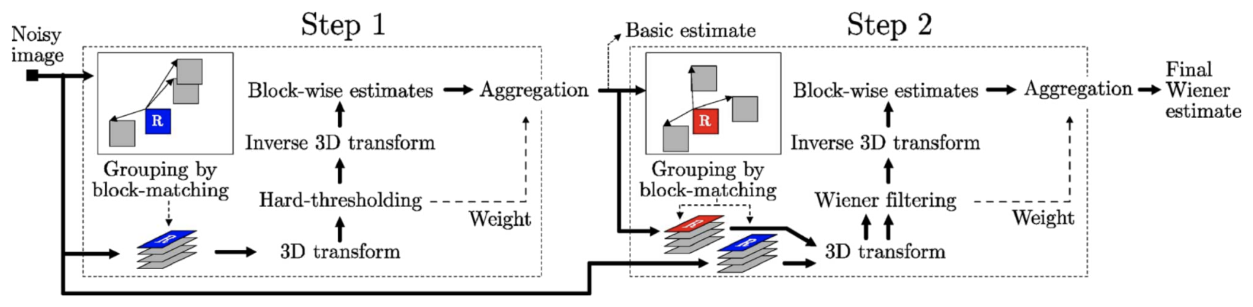
For roughly a decade after its publication, BM3D (Dabov et al. 2007) (slides 5–7) was the method to beat in Gaussian denoising. Its idea is non-local: natural images repeat themselves, so a small patch usually has many look-alikes elsewhere in the image (Figure 5.2). BM3D works in two stages, each with three steps (Figure 5.3).
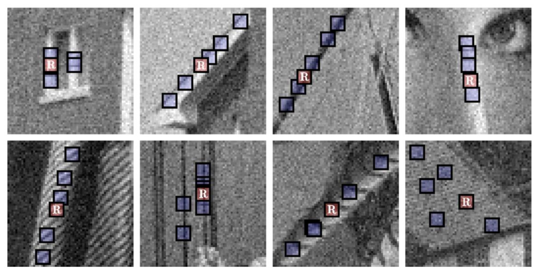
- Grouping by block matching. For a reference block R, search a window around it for blocks whose distance to R is below a threshold and stack them into a 3D array.
- Collaborative filtering. Apply a 3D decorrelating transform to the stack (a 2D transform within each block and a 1D transform across the stack), shrink the coefficients, and invert the transform. In stage 1 the shrinkage is hard thresholding; in stage 2 it is Wiener filtering, using the stage-1 output as a pilot estimate of the signal spectrum.
- Aggregation. Every pixel belongs to many groups, so it receives many estimates; these are averaged with weights that favour groups with less residual noise.
The lecture gave the intuition through principal components: in a stack of similar blocks, the content shared across blocks lives in a few leading components, while white noise spreads evenly over all of them, so keeping the leading components and discarding the rest removes mostly noise. (The original paper uses fixed transforms such as the DCT and a Haar transform across the stack rather than PCA, but the reasoning is the same.) On standard test images at \sigma = 25 (input PSNR 20.18 dB), BM3D reaches 32.08 dB on Lena and 30.73 dB on Barbara.
The lecture also pointed out a modern reading of BM3D. To process a block, it finds other blocks that are similar to it and processes them together. That is what an attention layer does: a query is compared against keys, and the most similar values are combined. BM3D hand-codes with signal processing what a transformer learns.
5.4 Supervised denoising and why it is not enough
5.4.1 The supervised objective
Given pairs (x, y) of clean and noisy images, the most direct approach (slide 8) trains a feed-forward network to map y to x:
\min_\Theta \mathbb{E}_{y \sim P_Y}\, \ell_{sup}(\Theta), \qquad \ell_{sup}(\Theta) = d(x, F_\Theta(y)) = \|x - F_\Theta(y)\|^2 , \tag{5.4}
and the trained network is used as \hat{x} = F_{\Theta^*}(y). It is the simplest and fastest method — one forward pass per image — and, as we will use repeatedly, its population minimizer is known in closed form.
Lemma 5.1 (The squared loss is minimized by the conditional mean) Let (x, y) be jointly distributed with \mathbb{E}\|x\|^2 < \infty. Among all measurable functions F, the risk \mathbb{E}\|x - F(y)\|^2 is minimized by F^*(y) = \mathbb{E}[x \mid y].
Proof. Write m(y) = \mathbb{E}[x \mid y] and expand around it:
\mathbb{E}\|x - F(y)\|^2 = \mathbb{E}\|x - m(y)\|^2 + \mathbb{E}\|m(y) - F(y)\|^2 + 2\,\mathbb{E}\big[(x - m(y))^\top (m(y) - F(y))\big].
Condition the cross term on y. Given y, the factor m(y) - F(y) is fixed, and \mathbb{E}[x - m(y) \mid y] = 0 by definition of m, so the cross term is zero. The first term does not depend on F and the second is non-negative and vanishes exactly when F = m (almost surely).
So a perfectly trained supervised denoiser computes the posterior mean, or minimum mean squared error (MMSE) estimate. Keep this in mind: every self-supervised method below will be judged by whether its minimizer is still \mathbb{E}[x \mid y].
5.4.2 DnCNN and residual learning
DnCNN (Zhang et al. 2017) (slides 9–10) made this work with a deep CNN. Its key design choice is residual learning: instead of predicting the clean image, the network \mathcal{R}(y; \Theta) predicts the noise y - x, and the loss over N training pairs is
\ell(\Theta) = \frac{1}{2N} \sum_{i=1}^N \big\| \mathcal{R}(y_i; \Theta) - (y_i - x_i) \big\|_F^2 , \tag{5.5}
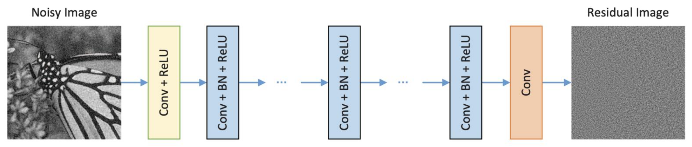
with the denoised image \hat{x} = y - \mathcal{R}(y; \Theta). The architecture is a plain stack: Conv+ReLU, then many Conv+BatchNorm+ReLU blocks, then a final Conv (Figure 5.4; this is the network we met in the batch-normalization lecture).
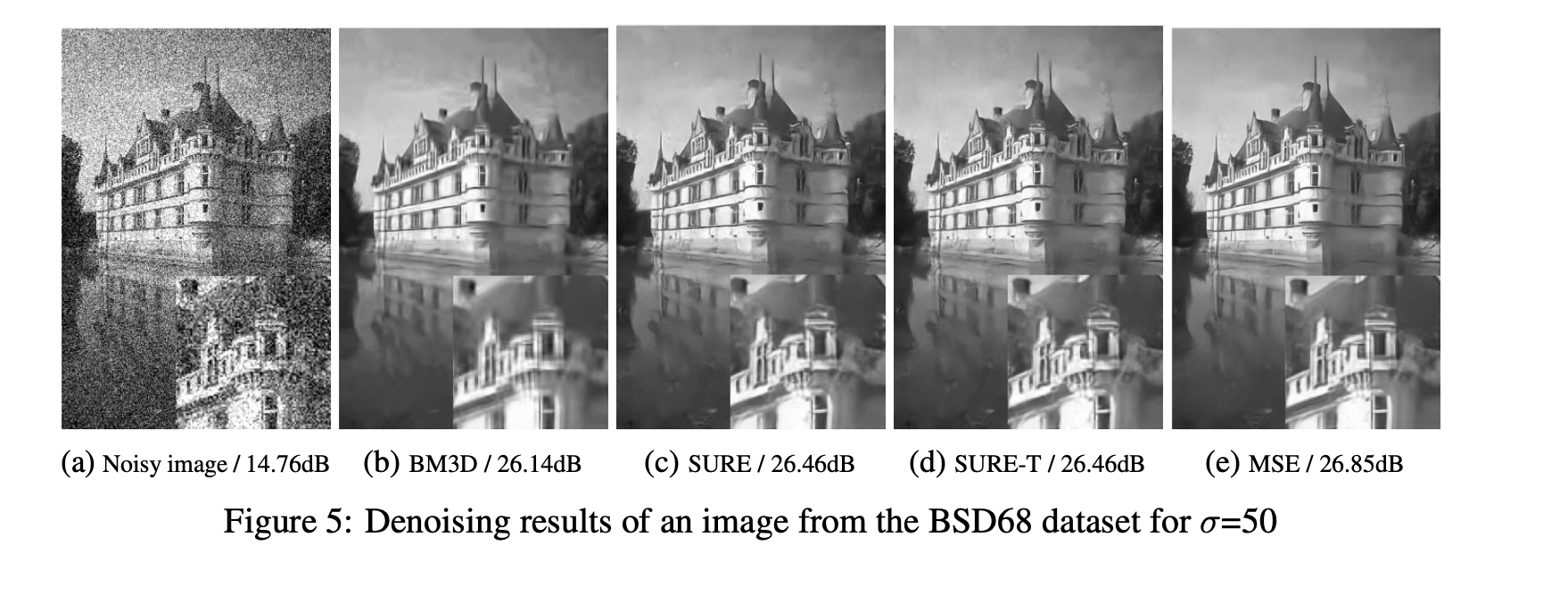
On the castle image at \sigma = 50 (input 14.76 dB) the slides report BM3D 26.21 dB, WNNM 26.51 dB, EPLL 26.36 dB and DnCNN 26.90–26.92 dB. The gains were real but modest, and on texture-rich images early supervised networks did not consistently beat BM3D, which led to some pessimism at the time about learned denoisers.
The lecture asked the class what Equation 5.5 reminds us of. A network that takes a noisy image and outputs the noise component is exactly the \epsilon-prediction network of a diffusion model (Ho et al. 2020). The difference is in what the network is used for: DnCNN is trained for one noise level (DnCNN-S) or a range of levels (the blind model DnCNN-B, \sigma \in [0, 55]) and is applied once, whereas a diffusion model is trained across a whole schedule of noise levels and is applied repeatedly to generate samples. When DnCNN appeared it was not clear why estimating the noise should be the right thing to do; Tweedie’s formula, below, gives the answer.
5.4.3 When clean targets do not exist
The weakness of Equation 5.4 is in its data: it requires matched clean images. In many scientific problems these do not exist.
- In the black-hole image of the Event Horizon Telescope, nobody has ever seen the object, so there is no ground truth at all.
- In cryo-electron microscopy (cryo-EM), the electron dose must be kept low to avoid destroying the specimen, so every image is very noisy (input SNR around 0 dB) and a clean version cannot be acquired.
- In live-cell or fast-moving imaging, the object moves between exposures, so even long exposures or averaging do not produce a clean reference.
Simulated noise is no escape, because real physical noise rarely matches the simulation. This motivates the question of the lecture: how can we train a denoiser without matched clean images?
5.5 Noise2Noise: learning from pairs of noisy images
5.5.1 The surprising observation
Noise2Noise (Lehtinen et al. 2018) (slides 12–13) replaces the clean target by a second noisy observation of the same image. With two measurements
y_1 = x + w_1, \qquad y_2 = x + w_2 ,
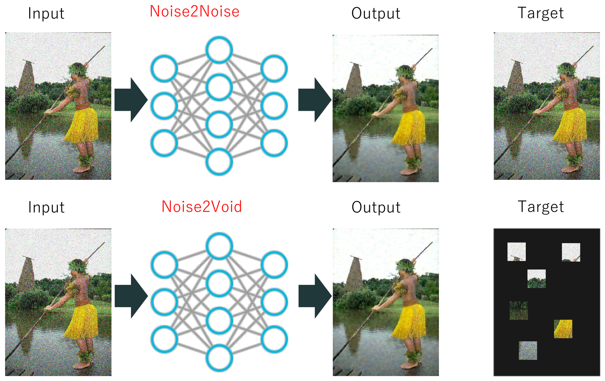
the network is trained to map one to the other (Figure 5.5, top):
\min_\Theta \; \mathbb{E}\, \|y_2 - F_\Theta(y_1)\|^2 . \tag{5.6}
One would expect the network to learn to reproduce noise, since that is what the targets contain. Instead, at test time it outputs a clean image, and the quality is almost that of supervised training: in the slides’ text-removal example the network trained on corrupted targets reaches 35.75 dB against 35.82 dB with clean targets.
5.5.2 Why the minimizer does not change
Theorem 5.1 (Noise2Noise has the supervised minimizer) Assume the second noise is conditionally zero-mean given the input, \mathbb{E}[w_2 \mid x, y_1] = 0, and that all second moments are finite. (This holds, in particular, when w_2 is independent of (x, w_1) and \mathbb{E}[w_2] = 0.) Then for every F,
\mathbb{E}\|y_2 - F(y_1)\|^2 = \mathbb{E}\|x - F(y_1)\|^2 + \mathbb{E}\|w_2\|^2 , \tag{5.7}
so the Noise2Noise loss and the supervised loss differ by a constant that does not depend on F, and both are minimized by F^*(y_1) = \mathbb{E}[x \mid y_1].
Proof. Substitute y_2 = x + w_2 and expand the square:
\mathbb{E}\|x + w_2 - F(y_1)\|^2 = \mathbb{E}\|x - F(y_1)\|^2 + \mathbb{E}\|w_2\|^2 + 2\,\mathbb{E}\big[(x - F(y_1))^\top w_2\big].
For the cross term, condition on (x, y_1). The vector x - F(y_1) is then fixed, so
\mathbb{E}\big[(x - F(y_1))^\top w_2\big] = \mathbb{E}\big[(x - F(y_1))^\top\, \mathbb{E}[w_2 \mid x, y_1]\big] = 0 .
This proves Equation 5.7. The minimizer of the right-hand side is \mathbb{E}[x \mid y_1] by Lemma 5.1.
Two remarks make the statement precise.
- What is needed is only that the noise in the target averages to zero given the input. The noise need not be Gaussian, need not be independent across pixels, and need not have the same distribution as w_1. In particular, \mathbb{E}[y_2 \mid y_1] = \mathbb{E}[x \mid y_1]: the network regresses on the noisy target, and the regression function of the noisy target coincides with that of the clean one.
- The price is variance, not bias. With finitely many training pairs, the noisy targets make the empirical loss a noisier estimate of the population loss, so more data are needed for the same accuracy.
5.5.3 Which loss recovers which statistic
The squared loss recovers the mean of the target distribution. Other losses recover other statistics, and Noise2Noise exploits this to handle noise that is not zero-mean. For a scalar random variable z consider c^* = \arg\min_c \mathbb{E}|z - c|^p.
- L_2 (p = 2): \frac{d}{dc}\mathbb{E}(z - c)^2 = -2(\mathbb{E}z - c) = 0 gives c^* = \mathbb{E} z, the mean.
- L_1 (p = 1): for a continuous z with CDF G, \mathbb{E}|z - c| = \int_{-\infty}^{c}(c - t)\,dG(t) + \int_c^\infty (t - c)\,dG(t), so \frac{d}{dc}\mathbb{E}|z - c| = G(c) - (1 - G(c)) = 2G(c) - 1. Setting it to zero gives G(c^*) = 1/2, the median.
- L_0 (mode seeking): for a discrete target the zero-one loss gives \mathbb{E}[\mathbf{1}\{z \ne c\}] = 1 - \Pr(z = c), so its minimizer is the most probable value, the mode. For a continuous target one maximizes instead \Pr(|z - c| \le h) for a small window h, which approaches a mode of the density as h \to 0 under regularity conditions. Noise2Noise implements this with the surrogate (|z - c| + \epsilon)^p and p annealed from 2 toward 0 during training; this is a practical mode-seeking device, not a theorem that the minimizer reaches the mode for every distribution.
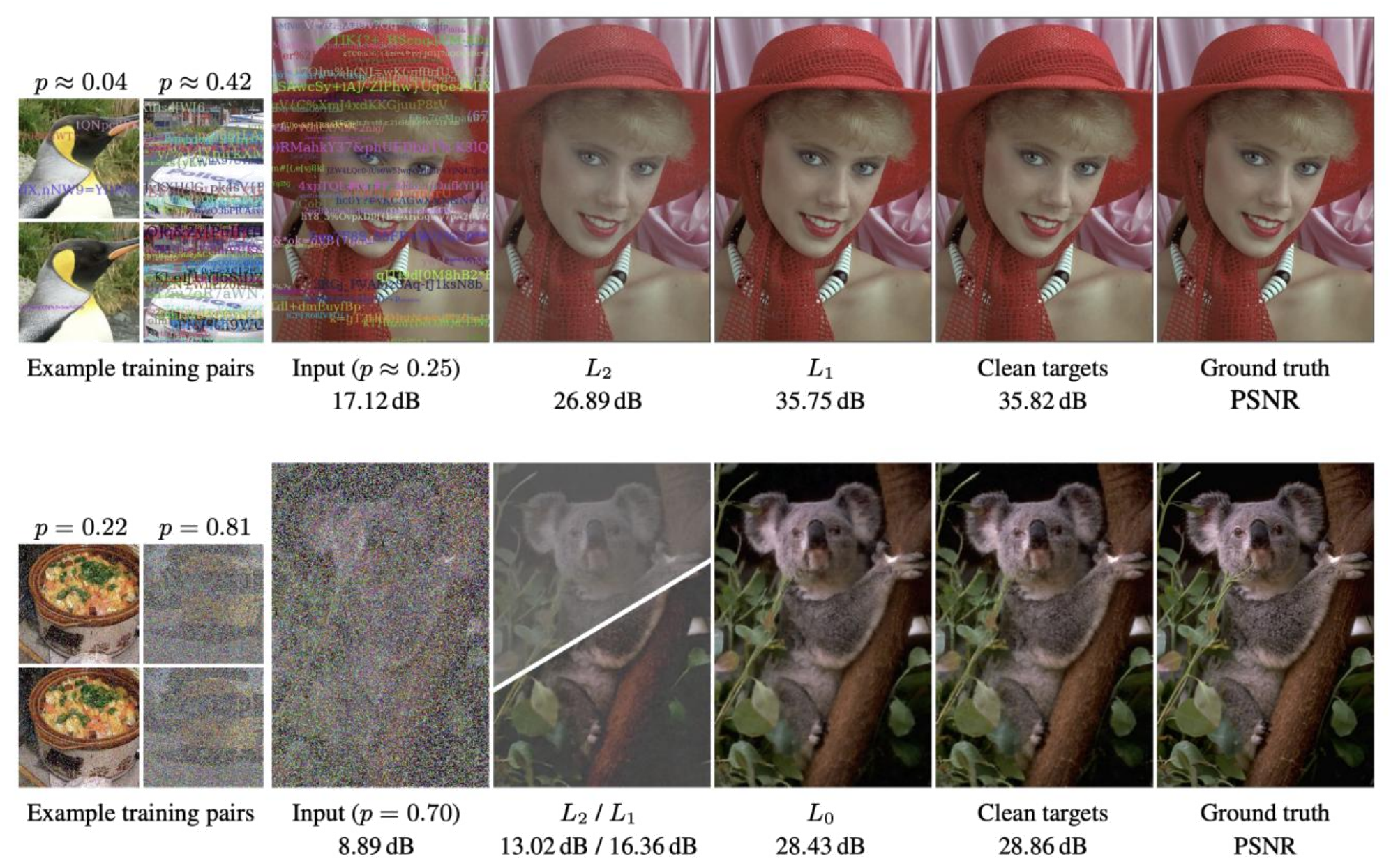
The text-removal and impulse-noise examples on slide 13 (Figure 5.6) show why this matters. A random text overlay replaces a fraction p of pixels by text colours; the corruption is not zero-mean, so the L_2 loss converges to the average of the clean colour and the text colours and leaves a visible shadow (26.89 dB at p \approx 0.25). When the clean colour is (nearly) determined by the input and p < 1/2, it is still the median of the target distribution at each pixel, so the L_1 loss recovers it (35.75 dB, against 35.82 dB with clean targets). For random-valued impulse noise at p = 0.70, even the median is corrupted (L_2/L_1 give 13.02/16.36 dB); but the clean value is still the single most likely value, so the annealed L_0 loss recovers the mode and reaches 28.43 dB, against 28.86 dB with clean targets.
One caution: the clean-target equivalence of Theorem 5.1 was proved for the squared loss only. For L_1 there is no general analogue, because adding independent zero-median noise to an uncertain clean value does not preserve its conditional median. The L_1 and L_0 results rely on the corruption leaving the relevant statistic of the target unchanged, which has to be checked for each corruption model.
5.5.4 The limitation
Noise2Noise removes the need for clean images, but it still needs two independent noisy observations of exactly the same scene. For a moving object, a dose-limited specimen or a one-off astronomical event, that is usually as hard to get as a clean image. The next question is therefore: can we train from a single noisy image?
5.6 Noise2Self, J-invariance and Noise2Void
5.6.1 Why a single noisy image is a problem
The obvious loss with a single image is the autoencoder loss \mathbb{E}\|y - F_\Theta(y)\|^2. It has a trivial minimizer: the identity F(y) = y achieves zero loss and removes no noise at all. Any single-image method must exclude the identity. Two ways are known: restrict the network so that it cannot see the pixel it predicts (this section), or add a penalty that makes copying expensive (SURE, next section).
5.6.2 J-invariance
The slides present this idea through Noise2Void; the formal argument below, from Noise2Self (Batson and Royer 2019), is added here because it explains why hiding a pixel rules out the identity. Let \mathcal{J} = \{J_1, \dots, J_K\} be a partition of the pixel indices \{1, \dots, n\}. For a subset J write y_J for the pixels in J and J^c for its complement.
Definition 5.1 (J-invariant function) A function F : \mathbb{R}^n \to \mathbb{R}^n is \mathcal{J}-invariant if for every J \in \mathcal{J} the output F(y)_J does not depend on the input y_J; that is, F(y)_J is a function of y_{J^c} only.
The identity is not \mathcal{J}-invariant, since F(y)_J = y_J depends on nothing but y_J. The point of the definition is the following identity.
Theorem 5.2 (Self-supervised loss for J-invariant functions) Suppose that, given x, the noisy pixels in different subsets are independent (y_J is conditionally independent of y_{J^c} given x, for each J \in \mathcal{J}), that the noise is zero-mean, \mathbb{E}[y \mid x] = x, and that second moments are finite. Then for every \mathcal{J}-invariant F,
\mathbb{E}\|F(y) - y\|^2 = \mathbb{E}\|F(y) - x\|^2 + \mathbb{E}\|y - x\|^2 . \tag{5.8}
Proof. Expand \|F(y) - y\|^2 = \|(F(y) - x) - (y - x)\|^2:
\mathbb{E}\|F(y) - y\|^2 = \mathbb{E}\|F(y) - x\|^2 + \mathbb{E}\|y - x\|^2 - 2 \sum_{J \in \mathcal{J}} \mathbb{E}\big[(F(y)_J - x_J)^\top (y_J - x_J)\big].
Fix one J and condition on x. By \mathcal{J}-invariance, F(y)_J - x_J is a function of (y_{J^c}, x) only; by assumption y_{J^c} and y_J are independent given x. The conditional expectation of the product therefore factorizes:
\mathbb{E}\big[(F(y)_J - x_J)^\top (y_J - x_J) \,\big|\, x\big] = \mathbb{E}\big[F(y)_J - x_J \,\big|\, x\big]^\top\, \mathbb{E}\big[y_J - x_J \,\big|\, x\big] = 0 ,
because \mathbb{E}[y_J \mid x] = x_J. Taking the outer expectation removes every cross term.
So, within the class of \mathcal{J}-invariant functions, minimizing the self-supervised loss on the noisy image is the same as minimizing the true error against the unseen clean image. Noise2Noise used independence between two images; Noise2Self uses independence between pixels of one image.
Note what the restriction costs. The best \mathcal{J}-invariant predictor of x_J is \mathbb{E}[x_J \mid y_{J^c}], not \mathbb{E}[x_J \mid y]: the network never uses the noisy value of the pixel it is predicting, which still carries information about that pixel. This is one reason blind-spot methods usually trail supervised training by a small margin.
5.6.3 Noise2Void: the blind-spot network in practice
Noise2Void (Krull et al. 2019) (slides 14–16) arrived at the same idea from the practical side, in the setting of microscopy. In a conventional CNN the receptive field of an output pixel contains the corresponding input pixel; a blind-spot network excludes it (Figure 5.7, left). Rather than designing such an architecture, Noise2Void trains an ordinary CNN with a masking scheme (Figure 5.7, right; target of Figure 5.5, bottom):
- pick a random set M of pixels in a training patch;
- replace each y_i, i \in M, by the value of a randomly chosen neighbour other than i itself, giving a modified input \tilde{y};
- compute the loss only on the masked pixels: \sum_{i \in M} (F_\Theta(\tilde{y})_i - y_i)^2.
Because the network never sees the original y_i at a masked location, it cannot copy it, and the argument of Theorem 5.2 applies to the masked pixels. In the lecture’s exaggerated picture, the network is shown an image with holes and learns to fill the holes from the context; because the noise in a hole is independent of its context, the best it can do is predict the clean value. One caveat: at test time the image is fed without masks, so the guarantee of Theorem 5.2 describes training; only an architectural blind spot keeps \mathcal{J}-invariance at inference.

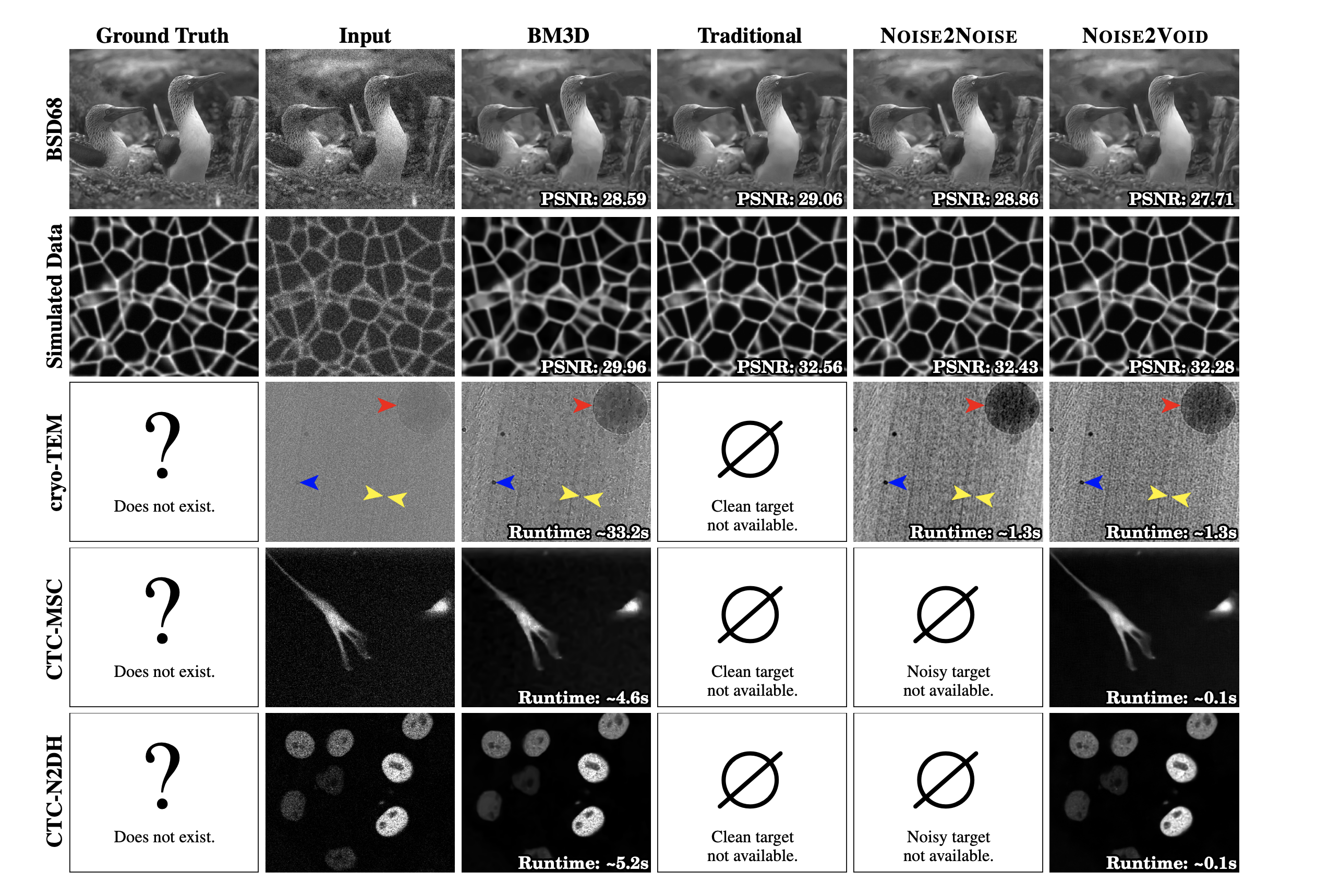
The slides compare Noise2Void with BM3D, supervised training (“traditional”) and Noise2Noise. On BSD68 the PSNRs are 28.59 (BM3D), 29.06 (supervised), 28.86 (Noise2Noise) and 27.71 dB (Noise2Void); on simulated cell-membrane data they are 29.96, 32.56, 32.43 and 32.28 dB. Noise2Void gives up a little accuracy, but it needs neither clean nor paired data. On real cryo-TEM and fluorescence data, where no clean target exists and often no second noisy copy either, only BM3D and Noise2Void are applicable at all, and Noise2Void is much faster at inference (about 0.1–1.3 s against 4.6–33.2 s for BM3D on the slides’ examples).
A student asked how the model knows which part of the image is noise. The answer is that it does not need to: the model assumes every pixel is signal plus noise, and the independence of the noise is the only thing that distinguishes the two. Under that independence assumption, whatever the network can predict from the context must come from the signal, because the noise at a pixel carries no information about its neighbours. When the noise is spatially correlated this breaks down, and the network also predicts the correlated part of the noise (see Section 5.12).
The lecture also asked what masking pixels and predicting them reminds us of. It is masked token prediction, as in masked language modelling (and, at the level of representations, JEPA). At the end of the lecture this resemblance is revisited as an analogy: both predict hidden content from its context, which for continuous images is tied to the score, while for discrete tokens it is an analogy rather than a theorem.
5.7 SURE: a single image with a divergence penalty
5.7.1 Stein’s unbiased risk estimate
The second way to exclude the identity keeps the plain autoencoder loss and adds a penalty. For Gaussian noise w \sim \mathcal{N}(0, \sigma^2 I), the SURE denoiser (Soltanayev and Chun 2018) (slides 17–19) minimizes
\ell_{SURE}(\Theta) = \mathbb{E}_{y \sim P_Y}\, d(y, F_\Theta(y)), \qquad d(y, F_\Theta(y)) := \|y - F_\Theta(y)\|^2 + 2\sigma^2 \operatorname{div}_y F_\Theta(y) . \tag{5.9}
The first term is the autoencoder loss; the second, the divergence-based penalty, is large for the identity, whose divergence is n. The construction comes from classical statistics, where Stein’s unbiased risk estimator (SURE) (Stein 1981) was used for decades, for example to tune wavelet thresholds, before deep learning. The key fact is Stein’s lemma.
Lemma 5.2 (Stein’s lemma) Let w \sim \mathcal{N}(0, \sigma^2 I_n) and let g : \mathbb{R}^n \to \mathbb{R}^n be weakly differentiable with \mathbb{E}|\partial g_i / \partial y_i| < \infty. Then, for fixed x and y = x + w,
\mathbb{E}\big[w^\top g(y)\big] = \sigma^2\, \mathbb{E}\big[\operatorname{div}_y g(y)\big].
Proof. It suffices to prove the scalar identity \mathbb{E}[w_i\, g_i(x + w)] = \sigma^2\, \mathbb{E}[\partial_i g_i(x + w)] for each coordinate and sum over i. Fix all coordinates except w_i; the density of w_i is \phi(t) = (2\pi\sigma^2)^{-1/2} e^{-t^2 / 2\sigma^2}, which satisfies t\, \phi(t) = -\sigma^2 \phi'(t). Integrating by parts,
\int t\, \phi(t)\, g_i(\dots, x_i + t, \dots)\, dt = -\sigma^2 \Big[\phi(t)\, g_i\Big]_{-\infty}^{\infty} + \sigma^2 \int \phi(t)\, \partial_i g_i(\dots, x_i + t, \dots)\, dt .
The boundary term vanishes under mild growth conditions (for example, if g_i grows at most polynomially; Stein (1981) gives the precise conditions). Taking the expectation over the other coordinates gives the claim.
Theorem 5.3 (SURE is unbiased for the true error) Under the assumptions of Lemma 5.2, and if \mathbb{E}\|F(y)\|^2 < \infty, for any fixed x,
\mathbb{E}\|F(y) - x\|^2 = \mathbb{E}\Big[\|y - F(y)\|^2 + 2\sigma^2 \operatorname{div}_y F(y)\Big] - n\sigma^2 . \tag{5.10}
Proof. Write F(y) - x = (F(y) - y) + w and expand:
\mathbb{E}\|F(y) - x\|^2 = \mathbb{E}\|F(y) - y\|^2 + 2\,\mathbb{E}\big[w^\top (F(y) - y)\big] + \mathbb{E}\|w\|^2 .
The last term is n\sigma^2. For the middle term, \mathbb{E}[w^\top y] = \mathbb{E}[w^\top x] + \mathbb{E}\|w\|^2 = n\sigma^2, and \mathbb{E}[w^\top F(y)] = \sigma^2\, \mathbb{E}[\operatorname{div}_y F(y)] by Stein’s lemma. Hence the middle term is 2\sigma^2 \mathbb{E}[\operatorname{div}_y F] - 2n\sigma^2, and collecting terms gives Equation 5.10.
As a sanity check, the identity F(y) = y has zero autoencoder loss but divergence n, so its SURE value is 2n\sigma^2 - n\sigma^2 = n\sigma^2, exactly the true error of not denoising: the penalty removes the identity’s artificial advantage. The right-hand side of Equation 5.10 can be evaluated without x. It is unbiased only in expectation; for one image it can even be negative, and a very flexible network can overfit it on a small dataset. The constant -n\sigma^2 does not affect the minimizer, which is why Equation 5.9 drops it. Because the identity holds for every fixed x, it also holds after averaging over x, so minimizing Equation 5.9 over networks is minimizing the supervised risk.
5.7.2 Computing the divergence: Monte-Carlo SURE
For a network with millions of outputs, \operatorname{div}_y F_\Theta is the trace of an n \times n Jacobian and cannot be formed explicitly. The SURE denoiser uses the Monte-Carlo estimate of Ramani et al. (2008): draw \tilde{n} \sim \mathcal{N}(0, I) independent of y and use, for a small \epsilon > 0,
\operatorname{div}_y F(y) \approx \frac{1}{\epsilon}\, \tilde{n}^\top \big(F(y + \epsilon \tilde{n}) - F(y)\big). \tag{5.11}
To see why, Taylor-expand F(y + \epsilon \tilde{n}) - F(y) = \epsilon\, J_F(y)\, \tilde{n} + O(\epsilon^2), where J_F is the Jacobian. Then the right-hand side of Equation 5.11 equals \tilde{n}^\top J_F(y)\, \tilde{n} + O(\epsilon), and since \mathbb{E}[\tilde{n}\tilde{n}^\top] = I,
\mathbb{E}_{\tilde{n}}\big[\tilde{n}^\top J_F(y)\, \tilde{n}\big] = \operatorname{tr}\big(J_F(y)\, \mathbb{E}[\tilde{n}\tilde{n}^\top]\big) = \operatorname{tr} J_F(y) = \operatorname{div}_y F(y) .
One extra forward pass per training step is enough; the randomness of \tilde{n} averages out over training like the randomness of a minibatch. Figure 5.14 checks both Equation 5.10 and Equation 5.11 numerically.
On one BSD68 image at \sigma = 50 (input 14.76 dB) the slides report BM3D 26.14 dB, a SURE-trained network 26.46 dB, and the same network trained with clean targets (MSE) 26.85 dB: SURE does not reach supervised quality, but it is close and it needs no clean data. Figure 5.9 is that comparison.
5.8 A side-by-side comparison
Slide 20 puts the three approaches next to each other.
- Supervised learning: \ell_{sup}(\Theta) = \|x - F_\Theta(y)\|^2, with noisy-clean pairs (x, y).
- Noise2X (Noise2Noise, Noise2Self, Noise2Void, …): \ell_{selfsup}(\Theta) = \|z - F_\Theta(y)\|^2, where the target z is derived from the noisy data in a way specific to each algorithm: a second noisy copy, the masked pixels, or (in Noisier2Noise (Moran et al. 2020)) the original y when the input is an even noisier version of it.
- SURE: \|y - F_\Theta(y)\|^2 + 2\sigma^2 \operatorname{div}_y F_\Theta(y), a divergence penalty compensating for the use of y itself as target.
Written this way, the losses differ mainly in the target (x, z or y), together with what each method adds to make that target usable: an independent second copy, a restriction on what the network may see, or the divergence penalty. These algorithmic choices look heuristic and unrelated, and each comes with its own proof. Is there a unified mathematical theory of self-supervised denoising — one that explains why all of them work and points to something better? The answer of Kim and Ye (2021) is Tweedie’s formula.
5.9 Tweedie’s formula
5.9.1 Exponential families and their posteriors
Following slides 22–23, a family of densities p(y \mid \eta) indexed by a parameter \eta is an exponential family if it can be written as
p(y \mid \eta) = p_0(y)\, \exp\!\big(\eta^\top T(y) - \varphi(\eta)\big), \tag{5.12}
where p_0(y) depends on y only, T(y) is the sufficient statistic, \eta is the natural parameter, and \varphi(\eta) depends on \eta only and makes the density integrate to one. The parameter enters only through the cross term \eta^\top T(y). Gaussian, Poisson, Gamma, Bernoulli and exponential distributions are all of this form, as the table in Section 5.9.6 shows. The decomposition is not unique (we will see two for the Gaussian), but the result below does not depend on the choice.
Put a prior p(\eta) on the parameter. Bayes’ rule gives the posterior
p(\eta \mid y) = \frac{p(y \mid \eta)\, p(\eta)}{p(y)} = \frac{p_0(y)}{p(y)}\, \exp\!\big(\eta^\top T(y)\big)\, e^{-\varphi(\eta)}\, p(\eta),
and absorbing p_0(y)/p(y) into the exponent,
p(\eta \mid y) = \exp\!\big(\eta^\top T(y) - \lambda(y)\big)\, \big[p(\eta)\, e^{-\varphi(\eta)}\big], \qquad \lambda(y) = \log \frac{p(y)}{p_0(y)} , \tag{5.13}
where p(y) = \int p(y \mid \eta) p(\eta)\, d\eta is the marginal density of the data. The posterior is itself an exponential family, now in \eta, with the roles of parameter and statistic exchanged: the cross term is again \eta^\top T(y), and the bracket depends only on \eta.
5.9.2 The closed form of the posterior mean
Under squared loss the Bayes-optimal estimate of \eta is the posterior mean \hat{\eta} = \mathbb{E}[\eta \mid y] (Lemma 5.1). The remarkable fact, due to Robbins and Tweedie and popularized by Efron (2011), is that this posterior mean can be written in terms of the marginal density of y alone.
Theorem 5.4 (Tweedie’s formula for exponential families) Let y be scalar, let p(y \mid \eta) have the form Equation 5.12 with T differentiable, and assume p(y) and p_0(y) are positive and differentiable and that differentiation in y may be exchanged with integration in \eta. Then
\hat{\eta}^\top T'(y) = \lambda'(y) = -\nabla_y \log p_0(y) + \nabla_y \log p(y) = -l_0'(y) + l'(y) , \tag{5.14}
where \hat{\eta} = \mathbb{E}[\eta \mid y] and T'(y) is the derivative of the sufficient statistic. The quantity l'(y) = \nabla_y \log p(y) is the score function of the noisy data.
Proof. The posterior Equation 5.13 integrates to one for every y:
\int \exp\!\big(\eta^\top T(y) - \lambda(y)\big)\, p(\eta)\, e^{-\varphi(\eta)}\, d\eta = 1 .
Differentiate both sides with respect to y. The bracket p(\eta) e^{-\varphi(\eta)} does not depend on y, and the derivative of the exponent is \eta^\top T'(y) - \lambda'(y), so
\int \big(\eta^\top T'(y) - \lambda'(y)\big)\, p(\eta \mid y)\, d\eta = 0 .
The first part of the integral is \mathbb{E}[\eta \mid y]^\top T'(y); the second is \lambda'(y) because p(\eta \mid y) integrates to one. Hence \hat{\eta}^\top T'(y) = \lambda'(y). Finally, \lambda(y) = \log p(y) - \log p_0(y) = l(y) - l_0(y), which gives the right-hand side of Equation 5.14.
Read Equation 5.14 from right to left. The noise model fixes T and p_0, which are known. The only thing that depends on the unknown clean-image distribution is the score l'(y) of the noisy data — and the noisy data are exactly what we have. If we can estimate the score from noisy images, we obtain the Bayes-optimal estimate of \eta without ever seeing a clean image.
For an image y \in \mathbb{R}^n with T(y) \in \mathbb{R}^k, the same proof differentiates with respect to each y_i. Writing J_T(y) \in \mathbb{R}^{k \times n} for the Jacobian of T, the result is
J_T(y)^\top\, \mathbb{E}[\eta \mid y] = \nabla_y \log p(y) - \nabla_y \log p_0(y). \tag{5.15}
When the noise acts independently on each pixel, J_T is (block) diagonal and this is the scalar formula applied pixel by pixel; the score \nabla_y \log p(y), however, still depends on the whole image, because the clean-image prior does not factorize. Two cautions follow from the form of Equation 5.15. The score determines \mathbb{E}[\eta \mid y] only through the linear map J_T^\top, which sends \mathbb{R}^k to \mathbb{R}^n; recovering an unrestricted k-dimensional \mathbb{E}[\eta \mid y] needs this map to be injective, i.e. \operatorname{rank} J_T = k (J_T has full row rank). Known components of \eta can supply the missing information, as for \eta_1 = \alpha - 1 in the Gamma case below. And \mathbb{E}[\eta(x) \mid y] is in general not \eta(\mathbb{E}[x \mid y]) when \eta is a nonlinear function of x; we meet both points in the Poisson and Gamma cases below.
5.9.3 Case 1: Gaussian noise
Let y = x + w with w \sim \mathcal{N}(0, \sigma^2) and \sigma known (slides 24–25). Expanding the square in the Gaussian likelihood separates the y-only, cross and x-only terms:
p(y \mid x) = \frac{1}{\sqrt{2\pi}\sigma} e^{-\frac{(y - x)^2}{2\sigma^2}} = \underbrace{\frac{1}{\sqrt{2\pi}\sigma} e^{-\frac{y^2}{2\sigma^2}}}_{p_0(y)} \exp\!\Big(\underbrace{\frac{x}{\sigma^2}}_{\eta}\, \underbrace{y}_{T(y)} - \underbrace{\frac{x^2}{2\sigma^2}}_{\varphi(\eta)}\Big).
So \eta = x/\sigma^2, T(y) = y with T'(y) = 1, and l_0(y) = -\frac{y^2}{2\sigma^2} + \text{const}, whence -l_0'(y) = y/\sigma^2. Substituting into Equation 5.14,
\mathbb{E}[\eta \mid y] = \frac{\hat{x}}{\sigma^2} = \frac{y}{\sigma^2} + l'(y),
and multiplying by \sigma^2,
\boxed{\;\hat{x} = \mathbb{E}[x \mid y] = y + \sigma^2\, l'(y), \qquad l'(y) = \nabla_y \log p(y).\;} \tag{5.16}
For an image with w \sim \mathcal{N}(0, \sigma^2 I) the same computation holds pixel by pixel, with l'(y) = \nabla_y \log p(y) \in \mathbb{R}^n. More generally, for correlated Gaussian noise w \sim \mathcal{N}(0, \Sigma) the vector decomposition \eta = \Sigma^{-1}x, T(y) = y, l_0(y) = -\frac{1}{2} y^\top \Sigma^{-1} y + \text{const} gives \Sigma^{-1}\hat{x} = \Sigma^{-1} y + \nabla_y \log p(y), that is \hat{x} = y + \Sigma\, \nabla_y \log p(y); we return to this when we discuss correlated noise.
The decomposition is not unique. The second Gaussian row of the table uses \eta = [x/\sigma^2, -1/(2\sigma^2)]^\top, T(y) = [y, y^2]^\top and p_0(y) = 1/\sqrt{2\pi}, so that l_0' = 0 and T'(y) = [1, 2y]^\top. Then Equation 5.14 reads \hat{x}/\sigma^2 - 2y/(2\sigma^2) = l'(y), which is again Equation 5.16. The term that was in p_0 has moved into \eta^\top T, and the answer is unchanged.
Denoising is score estimation. Equation 5.16 can be read in both directions:
l'(y) = \frac{\mathbb{E}[x \mid y] - y}{\sigma^2}, \qquad \mathbb{E}[w \mid y] = y - \mathbb{E}[x \mid y] = -\sigma^2\, l'(y). \tag{5.17}
An MMSE denoiser and the score of the noisy distribution determine each other. The second identity answers the question left open by DnCNN: a network trained to predict the noise from y converges to \mathbb{E}[w \mid y], which is the score scaled by -\sigma^2. Predicting noise, predicting the clean image and predicting the score are the same task. Figure 5.13 verifies Equation 5.16 on a two-component Gaussian mixture.
A direct check without exponential families. In the Gaussian case the formula can also be verified by differentiating the marginal p(y) = \int \mathcal{N}(y; x, \sigma^2 I)\, p(x)\, dx under the integral. Since \nabla_y \mathcal{N}(y; x, \sigma^2 I) = -\frac{y - x}{\sigma^2}\, \mathcal{N}(y; x, \sigma^2 I),
\nabla_y p(y) = \int \frac{x - y}{\sigma^2}\, \mathcal{N}(y; x, \sigma^2 I)\, p(x)\, dx \quad\Longrightarrow\quad \nabla_y \log p(y) = \frac{\mathbb{E}[x \mid y] - y}{\sigma^2},
after dividing by p(y) and recognising the posterior p(x \mid y) inside the integral. This is Equation 5.17 again, in any dimension.
A simple closed-form case. If x \sim \mathcal{N}(\mu, \tau^2), then y \sim \mathcal{N}(\mu, \tau^2 + \sigma^2) and l'(y) = -(y - \mu)/(\tau^2 + \sigma^2), so Tweedie gives \hat{x} = \frac{\tau^2}{\tau^2 + \sigma^2} y + \frac{\sigma^2}{\tau^2 + \sigma^2}\mu, the familiar Wiener shrinkage. With \mu = 0, \tau^2 = 4, \sigma^2 = 1 and y = 3, the score is -0.6 and \hat{x} = 3 + 1 \cdot (-0.6) = 2.4; the Bayes risk is \tau^2\sigma^2/(\tau^2 + \sigma^2) = 0.8 against 1 for the raw observation.
5.9.4 Case 2: Poisson noise
Photon-limited imaging (low-light fluorescence, astronomy, PET; slide 26) produces counts: y \in \{0, 1, 2, \dots\} with mean x > 0,
p(y \mid x) = \frac{x^y e^{-x}}{y!} = \underbrace{\frac{1}{y!}}_{p_0(y)} \exp\!\big(\underbrace{\log x}_{\eta}\cdot \underbrace{y}_{T(y)} - \underbrace{x}_{\varphi(\eta) = e^\eta}\big).
Here \eta = \log x, T(y) = y and T'(y) = 1. To differentiate in y we extend p(y) and p_0(y) smoothly to real y, using y! = \Gamma(y + 1). Then l_0(y) = -\log \Gamma(y + 1) and l_0'(y) = -\psi(y + 1), where \psi is the digamma function. The asymptotic expansion \psi(z) = \log z - \frac{1}{2z} + O(z^{-2}) gives \psi(y + 1) = \log(y + \frac{1}{2}) + O(y^{-2}), which is the approximation on the slides:
l_0'(y) \approx -\log\!\big(y + \tfrac{1}{2}\big).
Substituting into Equation 5.14 gives the exact relation and its approximation,
\mathbb{E}[\log x \mid y] = \psi(y + 1) + l'(y) \approx \log\!\big(y + \tfrac{1}{2}\big) + l'(y),
and writing \log \hat{x} for the right-hand side,
\boxed{\;\hat{x} = \big(y + \tfrac{1}{2}\big) \exp\!\big(l'(y)\big).\;} \tag{5.18}
One subtlety deserves to be stated. Tweedie’s formula gives the posterior mean of the natural parameter, here \log x. So Equation 5.18 is (approximately) \exp(\mathbb{E}[\log x \mid y]), the posterior geometric mean, which by Jensen’s inequality is never larger than \mathbb{E}[x \mid y]; the digamma approximation adds a further error at small counts. The worked example of Section 5.15.1.4 measures both gaps.
For comparison, the exact posterior mean of x also has a closed form in terms of the marginal, without any derivative (Robbins’ formula; see Efron (2011)). Since x \cdot \frac{x^y e^{-x}}{y!} = (y + 1)\frac{x^{y+1} e^{-x}}{(y+1)!},
(y + 1)\, p(y + 1) = \int x\, \frac{x^y e^{-x}}{y!}\, p(x)\, dx \quad\Longrightarrow\quad \mathbb{E}[x \mid y] = (y + 1)\, \frac{p(y + 1)}{p(y)} .
For counts, a ratio of neighbouring probabilities plays the role that the score plays for continuous data. Note that the two formulas estimate different quantities: Robbins’ ratio gives the arithmetic posterior mean exactly, whereas Equation 5.18 approximates the geometric one (compare the columns of Table 5.5 below).
5.9.5 Case 3: Gamma noise
Multiplicative noise — speckle in ultrasound and synthetic aperture radar, for instance — is modelled by a Gamma distribution whose scale is proportional to the clean value. Following slide 27, write
p(y \mid x) \propto \Big(\frac{y}{x}\Big)^{\alpha - 1} e^{-\beta \frac{y}{x}} = \exp\!\Big( (\alpha - 1)\log y - \frac{\beta}{x}\, y - (\alpha - 1)\log x \Big),
with \alpha, \beta known. This is the model y = x\, n with multiplicative noise n \sim \text{Gamma}(\alpha, \beta) (shape \alpha, rate \beta); the change of variables n = y/x contributes a factor 1/x, and the normalized density is
p(y \mid x) = \frac{\beta^\alpha}{\Gamma(\alpha)\, x^\alpha}\, y^{\alpha - 1} e^{-\beta y / x}, \qquad y > 0,
with \mathbb{E}[y \mid x] = \alpha x / \beta. The noise has mean one when \alpha = \beta = k, which is the setting “Gamma (k = 100)” of the experiments below. The x-only factors are absorbed in \varphi(\eta), which plays no role in Equation 5.14. The parameter enters through two cross terms, so \eta and T are vectors:
p_0(y) = 1, \qquad \eta = \begin{bmatrix} \alpha - 1 \\ -\beta / x \end{bmatrix}, \qquad T(y) = \begin{bmatrix} \log y \\ y \end{bmatrix}, \qquad T'(y) = \begin{bmatrix} 1/y \\ 1 \end{bmatrix}.
(The summary table on the slides lists T(y) = [\log y, -y]^\top; with \eta_2 = -\beta/x, the sign that reproduces e^{-\beta y / x} is T_2(y) = y, as on the derivation slide.) Since l_0' = 0, Equation 5.14 gives
\frac{\alpha - 1}{y} - \beta\, \mathbb{E}\Big[\frac{1}{x} \,\Big|\, y\Big] = l'(y).
Writing \beta/\hat{x} for \beta\,\mathbb{E}[1/x \mid y] and solving for \hat{x},
\boxed{\;\hat{x} = \frac{\beta y}{(\alpha - 1) - y\, l'(y)}.\;} \tag{5.19}
Here \hat{x} is the posterior harmonic mean, 1/\mathbb{E}[1/x \mid y], again because the natural parameter is -\beta/x rather than x. For an exact score the denominator (\alpha - 1) - y\, l'(y) = \beta y\, \mathbb{E}[1/x \mid y] is positive; with an estimated score it can approach zero or change sign, which an implementation has to guard against.
A conjugate example checks both the algebra and the interpretation. Take the prior x \sim \text{InverseGamma}(a_0, b_0), with density proportional to x^{-a_0 - 1} e^{-b_0 / x}. Multiplying by the likelihood gives the posterior \text{InverseGamma}(a_0 + \alpha,\, b_0 + \beta y), and integrating x out gives p(y) \propto y^{\alpha - 1} (b_0 + \beta y)^{-(a_0 + \alpha)}, so l'(y) = \frac{\alpha - 1}{y} - \frac{\beta (a_0 + \alpha)}{b_0 + \beta y}. With a_0 = 2, b_0 = 1, \alpha = \beta = 4 and y = 1: l'(1) = 3 - 4.8 = -1.8, and Equation 5.19 gives \hat{x} = 4/(3 + 1.8) = 5/6. The posterior is \text{InverseGamma}(6, 5), whose harmonic mean is b/a = 5/6 (exactly the formula) and whose mean is b/(a - 1) = 1.
5.9.6 The full table
Repeating the computation for other members of the family gives the table of Kim and Ye (2021) (slide 28). It is split here into the decompositions (Table 5.1) and the resulting estimators (Table 5.2), with the Gamma sign corrected and the Gamma density normalized as above.
| Distribution | p(y \mid x) | \eta | T(y) | p_0(y) |
|---|---|---|---|---|
| Gaussian | \frac{1}{\sqrt{2\pi}\sigma} e^{-\frac{(y-x)^2}{2\sigma^2}} | x/\sigma^2 | y | \frac{1}{\sqrt{2\pi}\sigma}e^{-\frac{y^2}{2\sigma^2}} |
| Gaussian (alt.) | same | [\frac{x}{\sigma^2}, -\frac{1}{2\sigma^2}]^\top | [y, y^2]^\top | \frac{1}{\sqrt{2\pi}} |
| Poisson | \frac{x^y e^{-x}}{y!} | \log x | y | \frac{1}{y!} |
| Gamma(\alpha, \beta) | \frac{\beta^\alpha y^{\alpha-1}}{\Gamma(\alpha) x^\alpha} e^{-\beta y/x} | [\alpha - 1, -\frac{\beta}{x}]^\top | [\log y, y]^\top | 1 |
| Bernoulli | x^y (1 - x)^{1 - y} | \log\frac{x}{1 - x} | y | 1 |
| Exponential | x e^{-yx}, y \ge 0 | -x | y | 1 |
| Distribution | l_0'(y) | Tweedie estimate \hat{x} | What \hat{x} is |
|---|---|---|---|
| Gaussian | -y/\sigma^2 | y + \sigma^2 l'(y) | posterior mean |
| Gaussian (alt.) | 0 | y + \sigma^2 l'(y) | posterior mean |
| Poisson | \approx -\log(y + \frac{1}{2}) | (y + \frac{1}{2}) \exp(l'(y)) | approx. posterior geometric mean |
| Gamma(\alpha, \beta) | 0 | \frac{\beta y}{(\alpha - 1) - y\, l'(y)} | posterior harmonic mean |
| Bernoulli | 0 | \frac{e^{l'(y)}}{1 + e^{l'(y)}} | logistic of posterior mean of \eta |
| Exponential | 0 | -l'(y) | posterior mean of the rate |
The last two rows are one line each. For the exponential distribution, p(y \mid x) = \exp(-x\, y + \log x), so \eta = -x, T = y, p_0 = 1, and Equation 5.14 gives \mathbb{E}[-x \mid y] = l'(y), i.e. \hat{x} = -l'(y); here \hat{x} is the genuine posterior mean of x because \eta is linear in x. For the Bernoulli distribution, \eta = \log\frac{x}{1-x} and \hat{\eta} = l'(y); mapping back through the inverse of the logit gives the sigmoid in the table (which, as in the Poisson case, is the image of the posterior mean of \eta, not the posterior mean of x; for a binary y the derivative must again be understood through a smooth extension).
The message of the table, highlighted on the slides, is: as long as we can compute the score function, optimal denoising can be achieved by Tweedie’s formula, for every noise model in the family. “Optimal” here has a precise meaning: the formula gives the posterior mean of the natural parameter, which is optimal for squared error in that parameter. It is the MMSE estimate of x itself when \eta is linear in x (Gaussian, exponential), and a geometric, harmonic or logistic posterior summary otherwise (Poisson, Gamma, Bernoulli).
5.10 Noise2Score
5.10.1 Training once, denoising by formula
Noise2Score (Kim and Ye 2021) (slide 29) turns the table into an algorithm with two phases.
- Training phase (noise-model agnostic). Train a network R_\Theta on noisy images only so that R_{\Theta^*}(y) \approx l'(y) = \nabla_y \log p(y).
- Inference phase (noise-model specific). Plug the estimated score into the Tweedie formula of Table 5.2 for the noise model at hand (Figure 5.10).
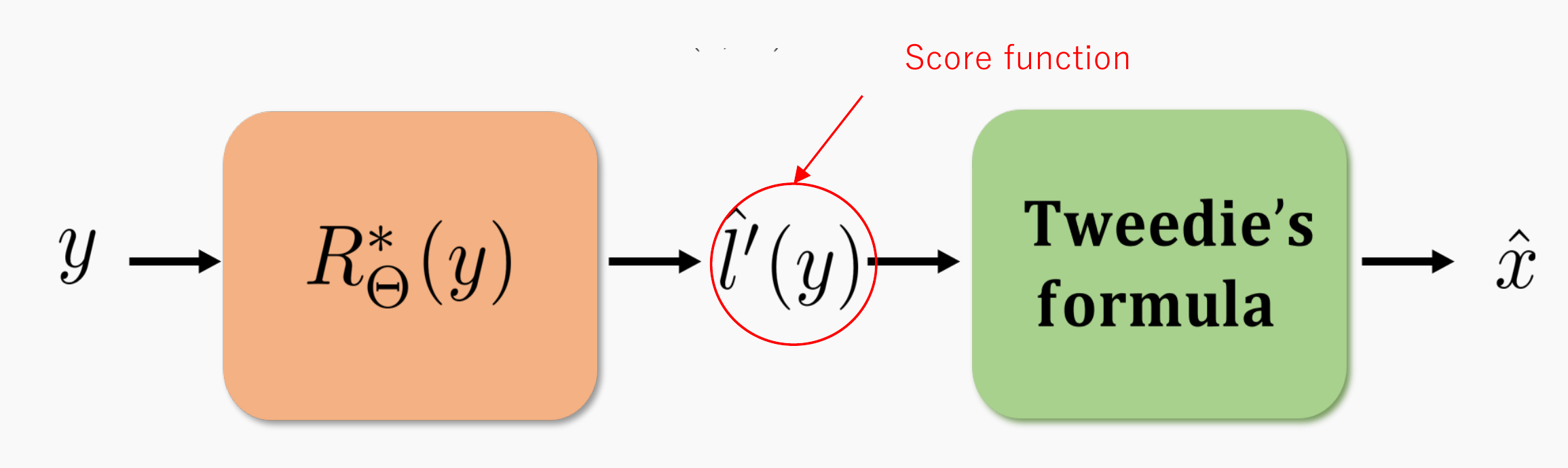
The noise model and its parameters (\sigma, or \alpha and \beta) enter only in the second phase, and the training procedure is the same whatever the noise. This should not be read as “one trained network serves every noise model”. The network learns the score of the observed distribution p(y), and p(y) depends on the noise: data with Poisson noise and data with Gaussian noise have different marginals and need their own score networks (or one network conditioned on the noise). What the separation buys is that, for a given dataset, the noise model is needed only at inference, and the same training code applies to every noise type.
This decomposition — learn the score of a distribution during training, design the downstream use at inference — is precisely the structure of diffusion models. There, too, training only learns a score, and sampling is a separate algorithm built on top of it; the difference is that diffusion sampling iterates (denoise with Tweedie, then add a little less noise), while Noise2Score denoises deterministically in one step. What remains is the training phase: how do we estimate the score from noisy samples?
5.11 Estimating the score from noisy data
5.11.1 The score function
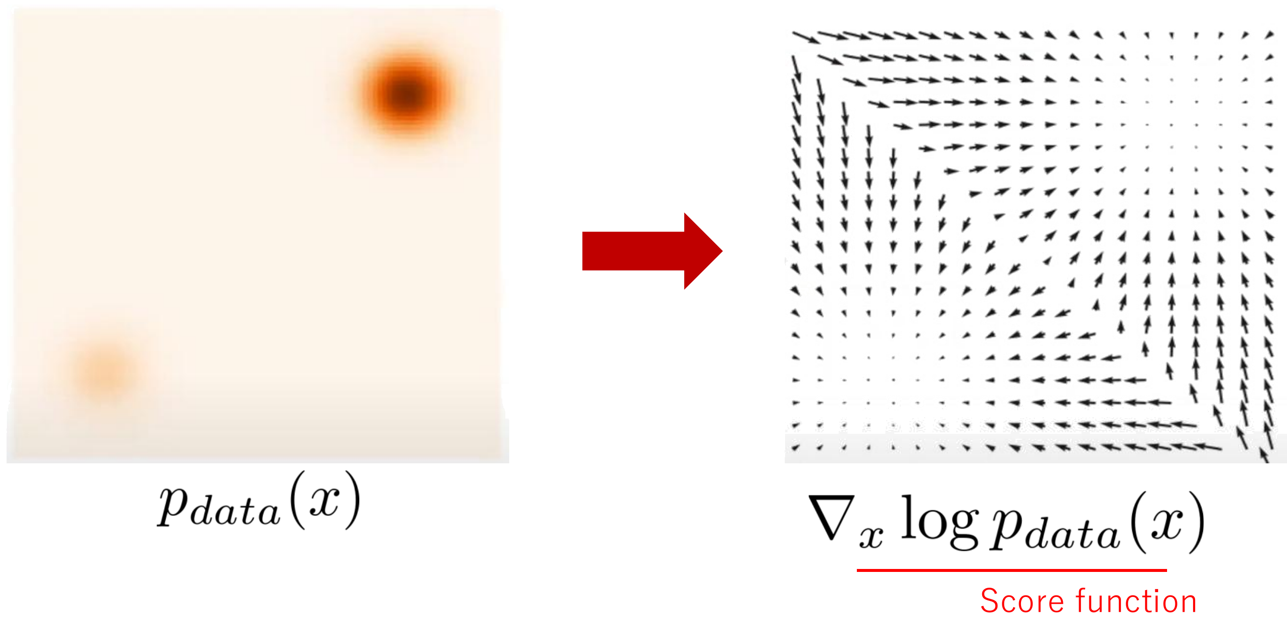
For a density p_{data}(x) (slide 31), the score \nabla_x \log p_{data}(x) is a vector field: at every point it points in the direction in which the density increases fastest, towards the nearby modes, with a magnitude that is large where the density changes quickly relative to its value (Figure 5.11). It is the same object that diffusion models learn. Two features make it convenient: it does not depend on the normalizing constant of p, since \nabla \log (c\, p) = \nabla \log p, and it can be estimated from samples. Before diffusion models, two classical estimators were known.
5.11.2 Denoising autoencoders estimate the score
The first is the denoising autoencoder (DAE). In the form shown on slide 32 (Alain and Bengio 2014), we take the noisy data y, corrupt it further with artificial Gaussian noise of level \sigma_a, and train the network to recover y:
\ell_{DAE}(\Theta) = \mathbb{E}_{\substack{y \sim P_Y \\ u \sim \mathcal{N}(0, I) \\ \sigma_a \sim \mathcal{N}(0, \delta^2)}} \big\| y - F_\Theta(y + \sigma_a u) \big\|^2 . \tag{5.20}
Note that this is a Noise2X loss: the input is a modified version of y, the target is y.
Proposition 5.1 (The optimal DAE is a score estimator) Fix the artificial noise level \sigma_a and let p_{\sigma_a} = p * \mathcal{N}(0, \sigma_a^2 I) be the density of \tilde{y} = y + \sigma_a u. The minimizer of Equation 5.20 at this level is
F_{\Theta^*}(\tilde{y}) = \tilde{y} + \sigma_a^2\, \nabla \log p_{\sigma_a}(\tilde{y}),
and as \sigma_a \to 0,
F_{\Theta^*}(y) = y + \sigma_a^2\, l'(y) + o(\sigma_a^2). \tag{5.21}
Proof. By Lemma 5.1 the minimizer is F^*(\tilde{y}) = \mathbb{E}[y \mid \tilde{y}]. The pair (y, \tilde{y}) is exactly a “clean signal plus Gaussian noise” pair, with y in the role of the clean signal and \sigma_a in the role of \sigma, so the Gaussian Tweedie formula Equation 5.16 applies to it with the marginal density p_{\sigma_a} of \tilde{y}: \mathbb{E}[y \mid \tilde{y}] = \tilde{y} + \sigma_a^2 \nabla \log p_{\sigma_a}(\tilde{y}). For the limit, p_{\sigma_a} solves the heat equation, so p_{\sigma_a} = p + \frac{\sigma_a^2}{2}\Delta p + o(\sigma_a^2) for smooth p, and therefore \nabla \log p_{\sigma_a} = \nabla \log p + O(\sigma_a^2). Multiplying by \sigma_a^2 gives Equation 5.21.
The score is then read off from the residual, \hat{l}'(y) = (F_{\Theta^*}(y) - y)/\sigma_a^2. Subtracting two nearly equal images and dividing by a tiny \sigma_a^2 is numerically fragile, so in practice the network is parameterized in residual form, F_\Theta(\tilde{y}) = \tilde{y} + \sigma_a^2 R_\Theta(\tilde{y}). For a fixed level \sigma_a, substituting \tilde{y} = y + \sigma_a u into Equation 5.20 gives
\ell_{DAE}(\Theta) = \sigma_a^2\, \mathbb{E}\, \big\| u + \sigma_a R_\Theta(y + \sigma_a u) \big\|^2 , \qquad R_{\Theta^*}(\tilde{y}) = -\frac{\mathbb{E}[u \mid \tilde{y}]}{\sigma_a} = \nabla \log p_{\sigma_a}(\tilde{y}),
so R_\Theta is trained directly as a score network. Three cautions keep the argument honest. First, at a fixed \sigma_a > 0 the DAE learns the score of the smoothed density p_{\sigma_a}, and only its rescaled residual converges to l' as \sigma_a \to 0; at \sigma_a = 0 the task is the plain autoencoder and the identity is optimal. Second, the slide samples \sigma_a \sim \mathcal{N}(0, \delta^2); a network that is not told \sigma_a then learns a weighted mixture of smoothed scores, so the fixed-scale result holds for it only approximately. Third, the auxiliary level \sigma_a is used only to learn the score; denoising the real image uses the physical noise level, \hat{x} = y + \sigma^2 R_{\Theta^*}(y), and confusing the two gives the wrong correction. Two further observations follow.
The limit is Tweedie for Gaussian noise. Equation 5.21 has exactly the form y + \sigma^2 l'(y) of Equation 5.16. The lecture asked the class where we had seen this formula before; this is the answer. A DAE trained at level \sigma_a outputs the Tweedie denoiser for Gaussian noise of level \sigma_a.
Noise2X methods are related to score estimation. Noisier2Noise (Moran et al. 2020) adds further noise to the noisy image and regresses back to it, which is the DAE loss with y as target; Moran et al. then apply a correction that depends on the noise model (for additive noise of the same level, 2F(z) - z) to reach the clean signal, and their method is not restricted to Gaussian noise. Noise2Noise has the same population minimizer as supervised training (Theorem 5.1), the MMSE denoiser, and for Gaussian noise that denoiser determines the score through Equation 5.17, so a perfectly trained Noise2Noise network is the Gaussian Tweedie denoiser. Blind-spot methods target the restricted conditional mean \mathbb{E}[x_J \mid y_{J^c}] instead, which is related to, but in general not equal to, the Tweedie denoiser. This is the sense in which the lecture explains these methods through the score.
As the lecture added, this reading is specific to Gaussian noise.
5.11.3 SURE is implicit score matching
The second classical estimator is score matching (Hyvarinen 2005) (slide 33). Plug the residual form
F_\Theta(y) = y + \sigma^2 R_\Theta(y), \qquad \hat{l}'(y) = \frac{F_{\Theta^*}(y) - y}{\sigma^2} = R_{\Theta^*}(y)
into the SURE loss Equation 5.9. (Slide 33 writes \sigma_a here; in SURE the level is the physical noise level \sigma, so we write \sigma.) The autoencoder term becomes \|y - F_\Theta(y)\|^2 = \sigma^4 \|R_\Theta(y)\|^2, and the divergence is \operatorname{div}_y F_\Theta = \operatorname{div}_y y + \sigma^2 \operatorname{div}_y R_\Theta = n + \sigma^2 \operatorname{div}_y R_\Theta. Hence
\begin{aligned} \ell_{SURE}(\Theta) &= \mathbb{E}_{y \sim P_Y}\big\{ \|y - F_\Theta(y)\|^2 + 2\sigma^2 \operatorname{div}_y F_\Theta(y) \big\} \\ &= \mathbb{E}_{y \sim P_Y}\big\{ \sigma^4 \|R_\Theta(y)\|^2 + 2\sigma^4 \operatorname{div}_y R_\Theta(y) \big\} + 2\sigma^2 n \\ &= 2\sigma^4\; \mathbb{E}_{y \sim P_Y}\Big\{ \tfrac{1}{2}\|R_\Theta(y)\|^2 + \operatorname{div}_y R_\Theta(y) \Big\} + 2\sigma^2 n . \end{aligned}
Up to the positive factor 2\sigma^4 and an additive constant, this is the implicit score matching loss of Hyvarinen (2005) with \Psi_\Theta = R_\Theta:
\ell_{ISM}(\Theta) = \mathbb{E}_{y \sim P_Y}\Big\{ \tfrac{1}{2}\|\Psi_\Theta(y)\|^2 + \operatorname{div}_y \Psi_\Theta(y) \Big\}. \tag{5.22}
Theorem 5.5 (Implicit score matching estimates the score) Assume that p > 0 is differentiable, that \Psi_\Theta is (weakly) differentiable, that \mathbb{E}\|\Psi_\Theta(y)\|^2, \mathbb{E}|\operatorname{div}_y \Psi_\Theta(y)| and \mathbb{E}\|\nabla_y \log p(y)\|^2 are finite, and that the boundary terms of the coordinatewise integration by parts vanish (for example, p(y)\Psi_\Theta(y) \to 0 as \|y\| \to \infty). Then
\ell_{ISM}(\Theta) = \tfrac{1}{2}\, \mathbb{E}_{y \sim P_Y} \|\Psi_\Theta(y) - \nabla_y \log p(y)\|^2 - \tfrac{1}{2}\, \mathbb{E}_{y \sim P_Y}\|\nabla_y \log p(y)\|^2 ,
so Equation 5.22 is minimized by \Psi_\Theta = \nabla_y \log p = l'.
Proof. Expand the square: \frac{1}{2}\mathbb{E}\|\Psi - \nabla \log p\|^2 = \frac{1}{2}\mathbb{E}\|\Psi\|^2 - \mathbb{E}[\Psi^\top \nabla \log p] + \frac{1}{2}\mathbb{E}\|\nabla \log p\|^2. For the middle term use p\, \nabla \log p = \nabla p and integrate by parts in each coordinate; the boundary terms vanish by assumption:
\mathbb{E}[\Psi^\top \nabla \log p] = \int \Psi(y)^\top \nabla p(y)\, dy = -\int \operatorname{div}\Psi(y)\, p(y)\, dy = -\mathbb{E}[\operatorname{div}\Psi] .
Substituting and rearranging gives the claim.
The boundary condition is not a formality to be waved through. Several of the noise models in Table 5.2 live on a half-line — Poisson, Gamma, exponential — and on a one-sided or bounded support the coordinatewise integration by parts leaves a term at the finite end as well, which has to be checked rather than discarded; it vanishes when p(y)\Psi_\Theta(y) \to 0 there too. The decay-at-infinity example above covers only the unbounded case.
So the SURE network, written in residual form, is trained to output the score, and the denoised image it produces is y + \sigma^2 l'(y), once more the Gaussian Tweedie formula (by Theorem 5.5). The lecture’s conclusion (slide 34): Noise2X and SURE are score-based approaches. For Gaussian noise, a DAE learns the score of a smoothed density, SURE in residual form learns the score of p(y) itself, and Noise2Noise learns the MMSE denoiser that is equivalent to that score; blind-spot methods learn a restricted version of the same conditional mean.
For Gaussian noise the link is exact in three places: any MMSE denoiser determines the score through Equation 5.17, a DAE identifies the score of the smoothed density, and SURE in residual form is implicit score matching. (The Noise2Noise and Noise2Self identities themselves do not need Gaussian noise; Gaussianity is what makes the conversion to a score simple.) The lecture extended the analogy to masked token prediction in language models and to diffusion models: in its reading, much of the success of modern self-supervised learning comes from the same decomposition into score estimation at training time and a well-designed downstream task at inference time. For discrete tokens this is an analogy between prediction tasks rather than a theorem about continuous image scores.
5.11.4 Results
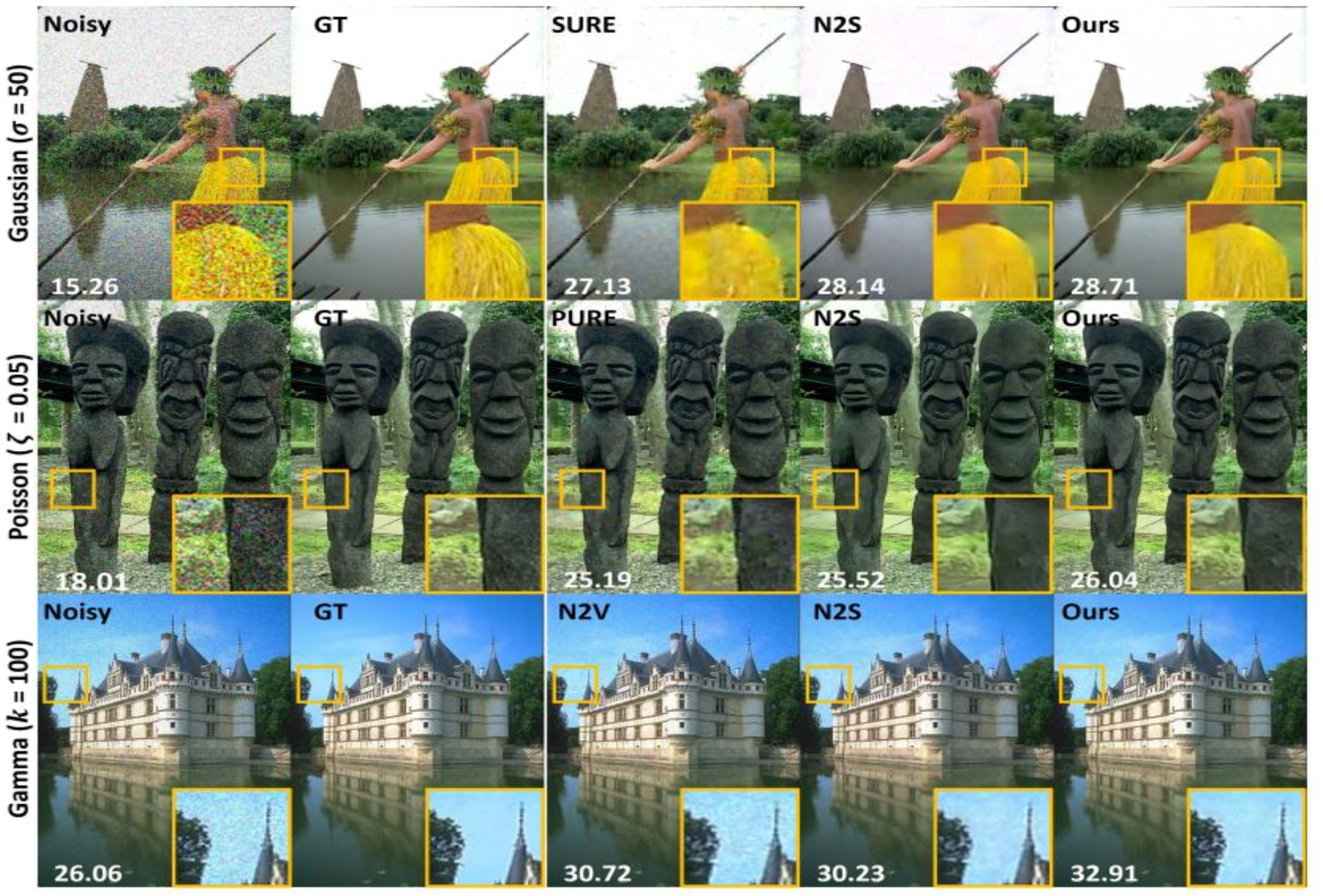
Because Noise2Score separates score estimation from the denoising formula, it can use the correct formula for each noise model. Slides 35–36 compare it with a noise-specific self-supervised baseline (SURE for Gaussian, its Poisson analogue PURE, Noise2Void for Gamma) and with Noise2Self. Figure 5.12 shows the first set of images and Table 5.3 collects the PSNR values of both slides.
| Noise | Image | Noisy | SURE / PURE / N2V | Noise2Self | Noise2Score |
|---|---|---|---|---|---|
| Gaussian, \sigma = 50 | 1 | 15.26 | 27.13 (SURE) | 28.14 | 28.71 |
| Gaussian, \sigma = 50 | 2 | 15.12 | 26.59 (SURE) | 27.60 | 28.18 |
| Poisson, \zeta = 0.05 | 1 | 18.01 | 25.19 (PURE) | 25.52 | 26.04 |
| Poisson, \zeta = 0.05 | 2 | 17.27 | 23.10 (PURE) | 23.65 | 24.45 |
| Gamma, k = 100 | 1 | 26.06 | 30.72 (N2V) | 30.23 | 32.91 |
| Gamma, k = 50 | 2 | 24.89 | 25.72 (N2V) | 26.82 | 29.47 |
The improvement over Noise2Self is about 0.6 dB for Gaussian noise and 0.5–0.8 dB for Poisson noise, and grows to about 2.7 dB for Gamma noise. These six images show the size of the gains; they do not by themselves establish the cause. Plausible contributors are that Noise2Score uses the noisy centre pixel that a blind-spot network discards, and that its reconstruction rule is matched to the noise model, but separating these would need ablations that the slides do not report. Since PSNR is 10\log_{10}(M^2/\text{MSE}) for a fixed peak M, a 2.68 dB gain means about 10^{0.268} \approx 1.85 times lower mean squared error. The lecture also pointed out that fine structures survive better: what used to be a collection of heuristics becomes one principled pipeline.
5.12 Where the independence assumption fails
Every identity in this chapter is carried by one assumption, and it is worth seeing them in one place before looking at what happens when they fail.
| Result | The assumption that carries the equality |
|---|---|
| Supervised squared error (Lemma 5.1) | the conditional expectation \mathbb{E}[x \mid y] exists |
| Noise2Noise (Theorem 5.1) | the target noise has zero conditional mean, \mathbb{E}[w_2 \mid x, y_1] = 0 |
| Noise2Self / Noise2Void (Theorem 5.2) | the hidden values are withheld from the network, and the noise is independent across the partition |
| SURE (Theorem 5.3) | additive Gaussian noise of known \sigma, and F_\Theta weakly differentiable with integrable divergence |
| Tweedie’s formula (Theorem 5.4) | the likelihood is a known exponential family, and the posterior normalization may be differentiated under the integral |
| DAE as score estimator (Proposition 5.1) | the perturbation is Gaussian, and the score is read in the limit \sigma_a \to 0 |
| Implicit score matching (Theorem 5.5) | the boundary terms of the integration by parts vanish |
Each fails in a recognizable way when it does not hold.
- Noise2Noise needs \mathbb{E}[w_2 \mid x, y_1] = 0. If the two copies share a noise component — fixed-pattern noise of a sensor, a common bias, a registration error between the shots — that component is predictable from y_1 and the network learns to reproduce it; Section 5.15.1.2 shows the optimum sliding from 0.8 to the identity as the correlation grows.
- Noise2Self and Noise2Void need the noise to be independent across the partition. Real camera noise is often spatially correlated after demosaicing, compression or the camera’s processing pipeline, and microscopy detectors can produce line or stripe artifacts. A blind-spot network then predicts the noise at a pixel from its correlated neighbours and leaves it in place. Structured masks that hide the whole correlated neighbourhood (Broaddus et al. 2020) are one remedy.
- SURE needs Gaussian noise with known \sigma; Stein’s lemma is a Gaussian identity.
- Tweedie’s formula and Noise2Score need a known likelihood. The formula in Table 5.2 is applied pixel by pixel, which presumes noise that is independent across pixels. For Gaussian noise with a known covariance \Sigma, the vector form \hat{x} = y + \Sigma\, \nabla_y \log p(y) derived above still holds; for unknown or non-exponential-family noise, the formula has to be rederived or the noise model estimated.
5.13 Connections and further reading
5.13.0.1 From denoising to diffusion models
The lecture closed with the bridge to diffusion models (slides 37–38). Tweedie’s formula holds at every noise level. A diffusion model adds controlled Gaussian noise of many levels to clean images, x_t = a_t x_0 + b_t \epsilon with \epsilon \sim \mathcal{N}(0, I) (a_t = 1, b_t = \sigma_t in the variance-exploding form; a_t = \sqrt{\bar{\alpha}_t}, b_t = \sqrt{1 - \bar{\alpha}_t} in DDPM), and trains one network to estimate the score \nabla \log p_t(x_t) of every noisy marginal. Applying Equation 5.16 to the clean signal a_t x_0 observed with noise level b_t,
\mathbb{E}[x_0 \mid x_t] = \frac{x_t + b_t^2\, \nabla_{x_t} \log p_t(x_t)}{a_t}, \qquad \mathbb{E}[\epsilon \mid x_t] = -b_t\, \nabla_{x_t} \log p_t(x_t),
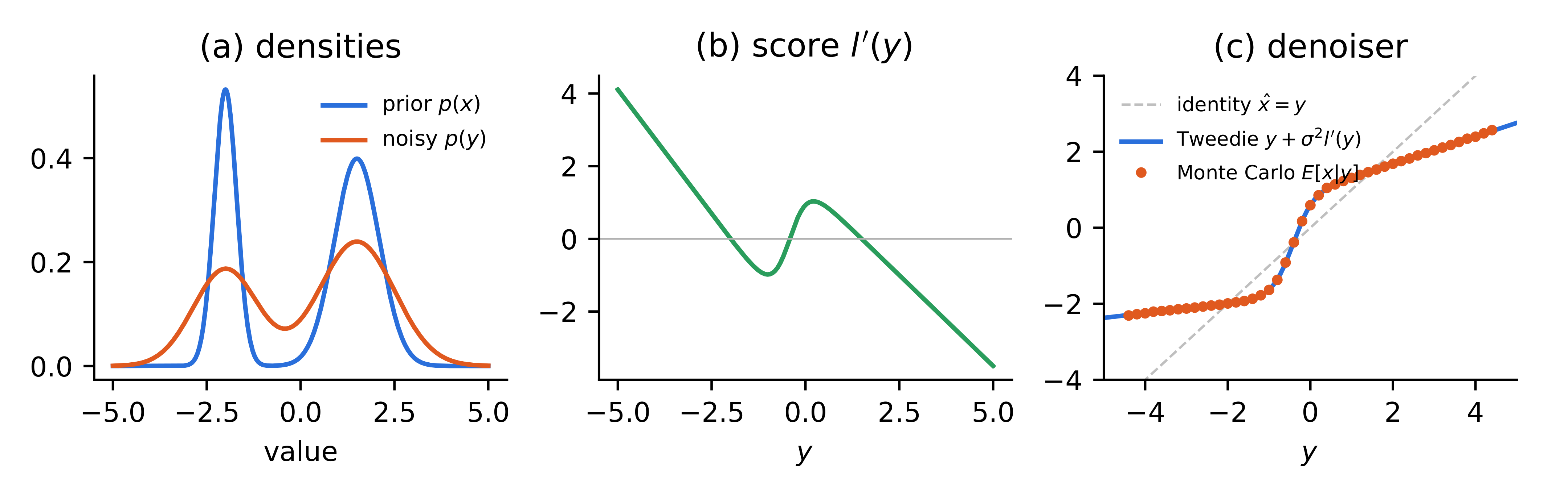
so the familiar \epsilon-prediction network of DDPM (Ho et al. 2020) is the same score, rescaled. Generation then becomes an iterative downstream task: estimate the clean image with Tweedie’s formula, add back a little less noise, and repeat (Song et al. 2021). A posterior mean is not a sample (Figure 5.13 (c) shows it falling between the modes), which is why the sampler needs the noise schedule and the stochastic or deterministic dynamics that later lectures specify. Self-supervised denoising is the one-step, deterministic special case of this machinery, and generalizing it beyond denoising is the topic of the next lecture.
5.13.0.2 Further reading
- Efron (2011) is a short, readable account of Tweedie’s formula and of empirical Bayes, including Robbins’ formula for counts.
- Batson and Royer (2019) develops \mathcal{J}-invariance beyond denoising (for example, for calibrating classical denoisers), and Broaddus et al. (2020) adapts the blind spot to spatially correlated noise.
- Moran et al. (2020) gives the Noisier2Noise correction for general additive and multiplicative noise.
- Vincent (2011) proves that denoising score matching and score matching are equivalent, which is the bridge from the DAE of slide 32 to the training objectives of Ho et al. (2020) and Song et al. (2021).
5.14 Summary
- Denoising is the inverse problem with \mathcal{A} = I. Classical methods regularize (sparsity, TV, RED, which are MAP estimates) or exploit non-local self-similarity (BM3D). Supervised networks such as DnCNN learn the posterior mean \mathbb{E}[x \mid y] but require clean targets.
- Noise2Noise trains on two independent noisy copies. Because the target noise is zero-mean given the input, the loss differs from the supervised loss by a constant (Theorem 5.1). The choice of loss selects the statistic: L_2 the mean, L_1 the median, L_0 the mode.
- Noise2Self / Noise2Void train on one noisy copy with a blind spot. \mathcal{J}-invariance excludes the identity, and independence of the noise across pixels makes the self-supervised loss equal to the true error plus a constant (Theorem 5.2).
- SURE trains on one noisy copy with a divergence penalty; Stein’s lemma makes it an unbiased estimate of the true error (Theorem 5.3), and the divergence is estimated by Monte Carlo.
- Tweedie’s formula expresses the posterior mean of the natural parameter of any exponential-family noise model through the score l'(y) of the noisy data (Theorem 5.4). For Gaussian noise, \mathbb{E}[x \mid y] = y + \sigma^2 l'(y): denoising is score estimation.
- Noise2Score learns the score of the observed data and applies the Tweedie formula matched to the noise model (Gaussian, Poisson, Gamma, …). For Gaussian noise, the population optimum of SURE in residual form is the score (for a network class that can represent it), that of Noise2Noise the equivalent MMSE denoiser, a DAE the score of a smoothed density, and blind-spot methods a restricted conditional mean; this is the lecture’s unified explanation of why they work. Noise2Noise and Noise2Self themselves do not require Gaussian noise.
- Learning a score at training time and using it through Tweedie’s formula at inference time is the core of diffusion models.
5.15 Advanced topics
The lecture states the results below; what follows works them through with numbers, and adds one example that points at the next chapter. None of it is needed to follow the argument above.
5.15.1 Worked examples
Unlike the PSNR values above, which are copied from the slides, the examples in this section are original to this note. Each is small enough to reproduce exactly, and each ends with a short, self-contained NumPy/SciPy snippet that prints the numbers quoted in the text, with the seeds used for the figures (the figures add only plotting calls).
5.15.1.1 Tweedie’s formula on a Gaussian mixture
Let the clean signal be a two-component Gaussian mixture, p(x) = 0.4\, \mathcal{N}(x; -2, 0.3^2) + 0.6\, \mathcal{N}(x; 1.5, 0.6^2), and observe y = x + w with \sigma = 0.8. Convolving each component with the noise gives the noisy marginal in closed form,
p(y) = \sum_k \pi_k\, \mathcal{N}(y; \mu_k, s_k^2 + \sigma^2), \qquad l'(y) = \frac{\sum_k \pi_k\, \mathcal{N}(y; \mu_k, s_k^2 + \sigma^2)\, \frac{\mu_k - y}{s_k^2 + \sigma^2}}{\sum_k \pi_k\, \mathcal{N}(y; \mu_k, s_k^2 + \sigma^2)},
with (\pi_k, \mu_k, s_k) the mixture weights, means and standard deviations. We draw 4 \times 10^5 pairs (x, y), estimate \mathbb{E}[x \mid y] by averaging x in narrow bins of y, and compare with y + \sigma^2 l'(y) (Figure 5.13). Over the 45 bins of width 0.2 between -4.5 and 4.5 (bins with fewer than 50 samples skipped), the largest discrepancy is 0.025, which reflects Monte-Carlo error together with the bias of comparing a bin average with the value at the bin centre. The denoiser is strongly nonlinear: near each mode it shrinks y towards that mode, and between the modes it switches quickly from one to the other. This is exactly what the score does in panel (b), where it changes sign at each mode and between them.
The following code reproduces the numbers above; Figure 5.13 is plotted from the same arrays.
import numpy as np
from scipy.stats import norm

#-- 1. Tweedie on a Gaussian mixture (Figure: tweedie-1d)
rng = np.random.default_rng(1)
pi = np.array([0.4, 0.6]); mu = np.array([-2.0, 1.5])
s = np.array([0.3, 0.6]); sig = 0.8
v = s**2 + sig**2                        # variances of p(y)

def score(y):                            # l'(y) = d/dy log p(y)
    w = pi * norm.pdf(y[:, None], mu, np.sqrt(v))
    return (w * (mu - y[:, None]) / v).sum(1) / w.sum(1)

k = rng.choice(2, 400_000, p=pi)
x = rng.normal(mu[k], s[k])
y = x + sig * rng.normal(size=x.size)
edges = np.linspace(-4.5, 4.5, 46)       # bins of width 0.2
centre = 0.5 * (edges[1:] + edges[:-1])
b = np.digitize(y, edges)
mc = np.array([x[b == i].mean() if (b == i).sum() > 50 else np.nan
               for i in range(1, len(edges))])
tw = centre + sig**2 * score(centre)
print("1. max |Tweedie - MC| =", np.nanmax(np.abs(tw - mc)))
5.15.1.2 Three objectives, one optimum — and what correlation does
A scalar model shows Theorem 5.1 and Theorem 5.3 in closed form and also shows the failure mode of Noise2Noise quantitatively. Let x \sim \mathcal{N}(0, 4), observe y = x + w_1 and a second copy z = x + w_2 with w_1, w_2 \sim \mathcal{N}(0, 1) independent, and restrict the denoiser to F_a(y) = a y. Expanding each objective,
\begin{aligned} \text{supervised:}\quad & \mathbb{E}(a y - x)^2 = 4(a - 1)^2 + a^2, \\ \text{Noise2Noise:}\quad & \mathbb{E}(a y - z)^2 = 4(a - 1)^2 + a^2 + 1, \\ \text{SURE:}\quad & \mathbb{E}\big[(a y - y)^2 + 2a\big] - 1 = 5(a - 1)^2 + 2a - 1 = 4(a - 1)^2 + a^2 , \end{aligned}
using \mathbb{E}y^2 = 5 and \operatorname{div} F_a = a. All three are minimized at a^* = 4/5, the Tweedie/Wiener coefficient \tau^2/(\tau^2 + \sigma^2). The Noise2Noise loss is larger by exactly \mathbb{E}w_2^2 = 1 (Equation 5.7), so comparing raw training-loss values across objectives is meaningless; only the minimizers agree.
Now let the two noises be correlated, \mathbb{E}[w_1 w_2] = \rho. The cross term of Theorem 5.1 no longer vanishes:
\mathbb{E}(a y - z)^2 = 4(a - 1)^2 + a^2 + 1 - 2a\rho, \qquad a^*_\rho = \frac{4 + \rho}{5}.
At \rho = 0.6 the optimum moves to 0.92, and at \rho = 1 (the two copies share their noise) it is a = 1, the identity: Noise2Noise then learns to copy its input. This is the independence condition of Theorem 5.1 failing in a measurable way.
The optima can be checked in one line each:
#-- 2. Scalar model: three objectives, correlated noise (exact)
for rho in (0.0, 0.6, 1.0):
    print("2. rho =", rho, " a* =", (4 + rho) / 5)
5.15.1.3 SURE without the clean image
Take a sparse vector x \in \mathbb{R}^{2000} with 200 nonzero entries drawn from \mathcal{N}(0, 4^2), observe y = x + w with \sigma = 1, and denoise by soft thresholding, F(y)_i = \operatorname{sign}(y_i)\max(|y_i| - \tau, 0). Its divergence is available in closed form, \operatorname{div}_y F = \#\{i : |y_i| > \tau\}, because each output coordinate has derivative 1 where it is not thresholded and 0 where it is. Figure 5.14 plots, as functions of \tau, the true error (which uses x), SURE Equation 5.10 with the exact divergence, and SURE with the Monte-Carlo divergence Equation 5.11 using a single probe (\epsilon = 10^{-3}). On a grid of \tau with step 0.05, the three curves track each other. The true optimum is \tau = 1.25 with error 0.254 per entry; SURE with the exact divergence picks the same \tau = 1.25, and the one-probe Monte-Carlo version picks \tau = 1.10, whose true error (0.262) is within 0.01 of the optimum. SURE picks a near-optimal denoiser from the noisy data alone.
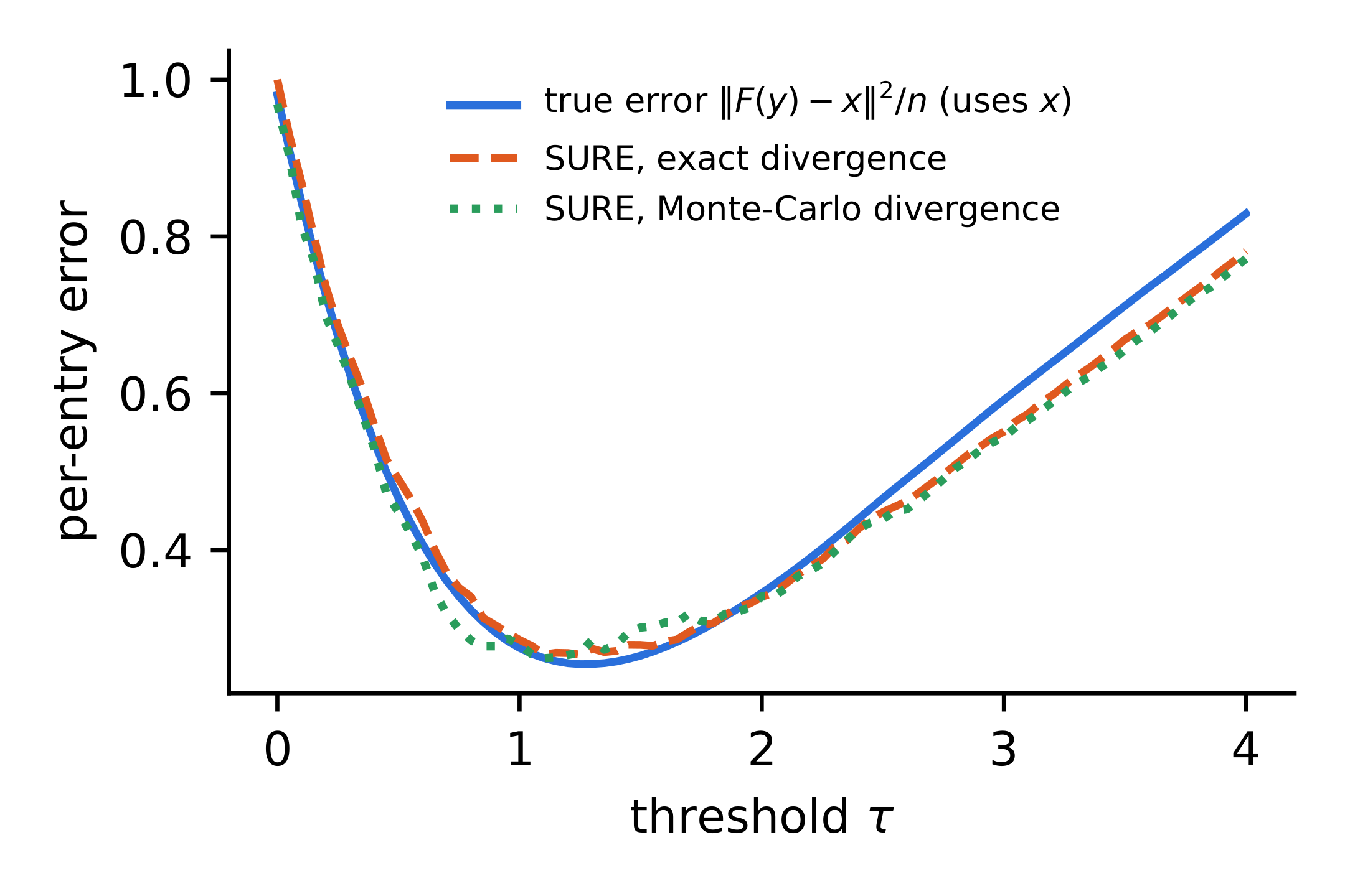
The code below produces the numbers in the text and the curves of Figure 5.14.
import numpy as np

#-- 3. SURE for soft thresholding (Figure: sure-check)
rng = np.random.default_rng(4)
d, sg = 2000, 1.0
xs = np.zeros(d)
xs[rng.choice(d, 200, replace=False)] = rng.normal(0, 4, 200)
ys = xs + sg * rng.normal(size=d)
probe, eps = rng.normal(size=d), 1e-3
soft = lambda u, t: np.sign(u) * np.maximum(np.abs(u) - t, 0)
taus = np.linspace(0, 4, 81)             # grid with step 0.05
true, sure, sure_mc = [], [], []
for t in taus:
    F = soft(ys, t)
    fit_term = np.sum((ys - F) ** 2) - d * sg**2
    div_mc = probe @ (soft(ys + eps * probe, t) - F) / eps
    true.append(np.sum((F - xs) ** 2) / d)
    sure.append((fit_term + 2 * sg**2 * np.sum(np.abs(ys) > t)) / d)
    sure_mc.append((fit_term + 2 * sg**2 * div_mc) / d)
for name, c in (("true", true), ("SURE", sure), ("MC-SURE", sure_mc)):
    i = int(np.argmin(c))
    print("3.", name, "tau* =", taus[i], " true error there =",
          round(true[i], 4))
5.15.1.4 How good is the Poisson formula?
With a Gamma prior on the Poisson rate everything is available in closed form, which lets us measure the error of Equation 5.18 exactly. Let x \sim \text{Gamma}(a, b) (shape a, rate b) and y \mid x \sim \text{Poisson}(x). The posterior is \text{Gamma}(a + y, b + 1), so
\mathbb{E}[x \mid y] = \frac{a + y}{b + 1}, \qquad \exp\!\big(\mathbb{E}[\log x \mid y]\big) = \frac{e^{\psi(a + y)}}{b + 1}.
The marginal of y is negative binomial; extending it to real y through the Gamma function, l(y) = \log\Gamma(a + y) - \log\Gamma(y + 1) - \log\Gamma(a) + a \log\frac{b}{b+1} - y\log(b + 1), so l'(y) = \psi(a + y) - \psi(y + 1) - \log(b + 1). For a = 4, b = 0.5:
| y | \mathbb{E}[x \mid y] | \exp(\mathbb{E}[\log x \mid y]) | (y + \frac{1}{2})\exp(l'(y)) |
|---|---|---|---|
| 0 | 2.667 | 2.341 | 2.085 |
| 1 | 3.333 | 3.006 | 2.955 |
| 2 | 4.000 | 3.672 | 3.648 |
| 5 | 6.000 | 5.670 | 5.662 |
| 10 | 9.333 | 9.002 | 8.999 |
| 20 | 16.000 | 15.668 | 15.666 |
Three things are visible in Table 5.5 and Figure 5.15. First, the formula is essentially exact for what it estimates, the geometric mean \exp(\mathbb{E}[\log x \mid y]), except at the smallest counts, where the approximation \psi(y + 1) \approx \log(y + \frac{1}{2}) is crude. Second, the geometric mean sits below the arithmetic posterior mean by an almost constant amount, here about 1/(2(b+1)) = 0.33, as predicted by \psi(z) \approx \log z - \frac{1}{2z}. Third, the posterior mean pulls the raw count towards the prior mean a/b = 8 (up for y < 8, down for y > 8); the other two columns are offset below it, so near y = 8 they sit slightly below both the count and the prior mean.
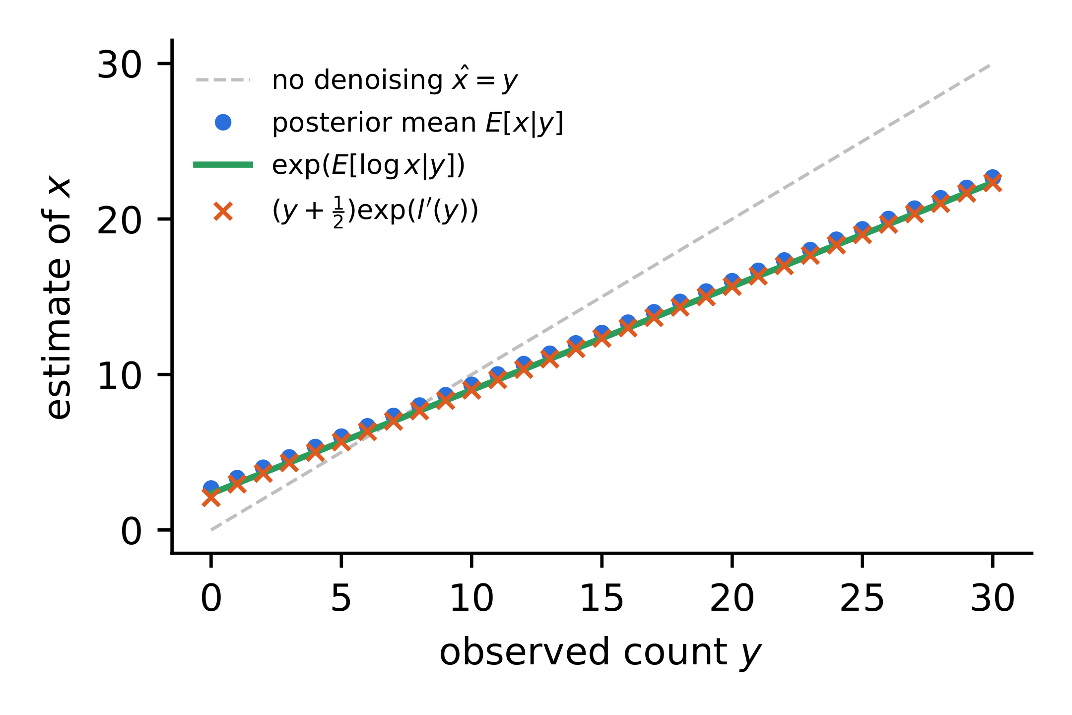
The code below produces Table 5.5.
import numpy as np
from scipy.special import digamma

#-- 4. Poisson Tweedie vs exact posterior, Gamma(4, 0.5) prior (exact)
a, bb = 4.0, 0.5
yy = np.arange(0, 31)
lp = digamma(a + yy) - digamma(yy + 1) - np.log(bb + 1)   # l'(y)
post_mean = (a + yy) / (bb + 1)
geo_mean = np.exp(digamma(a + yy)) / (bb + 1)
slide = (yy + 0.5) * np.exp(lp)
for j in (0, 1, 2, 5, 10, 20):
    print("4. y=%2d  %.3f  %.3f  %.3f"
          % (j, post_mean[j], geo_mean[j], slide[j]))
5.15.2 Tweedie’s formula on a DDPM forward marginal
One application is worth writing out because the next chapter opens with it. A single step of the DDPM forward process produces
y = \sqrt{\bar\alpha_t}\, x_0 + \sqrt{1 - \bar\alpha_t}\, \epsilon, \qquad \epsilon \sim \mathcal{N}(0, I), \tag{5.23}
with a mixing coefficient \bar\alpha_t \in (0,1], so that conditionally on x_0 the observation is Gaussian with mean \sqrt{\bar\alpha_t}\,x_0 and variance 1-\bar\alpha_t. Reading \sqrt{\bar\alpha_t}\,x_0 as the clean signal and 1-\bar\alpha_t as the noise variance, the Gaussian case of Equation 5.16 gives
\sqrt{\bar\alpha_t}\; \mathbb{E}[x_0 \mid y] = y + (1 - \bar\alpha_t)\, \nabla_y \log p_t(y), \qquad\text{so}\qquad \mathbb{E}[x_0 \mid y] = \frac{y + (1 - \bar\alpha_t)\, \nabla_y \log p_t(y)}{\sqrt{\bar\alpha_t}}, \tag{5.24}
where p_t is the marginal density of the noisy variable at time t.
Nothing here is new: it is the identity of Equation 5.16 with the variance read off a particular forward process. What it shows is that the quantity a diffusion model spends its training budget estimating — the score of a noisy marginal — is the same quantity this chapter has been estimating, and that recovering the clean signal from it is a formula rather than a second network.
Based on the scribe note of Hyeonjae Kim, with material from Donggyu Kim, Mingeon Kim and Jeonghun Lee; edited by Jong Chul Ye.