2 GAN and its Extensions
2.1 Overview
A generative adversarial network (GAN) learns to sample from an unknown data distribution without writing down a likelihood. A generator turns noise into samples, a discriminator tries to tell those samples from real data, and the two are trained against each other. The previous lecture introduced statistical distances and optimal transport; this lecture shows that every GAN variant is, underneath, a choice of statistical distance between the data and the model, together with a way of estimating that distance with a neural network.
The original GAN minimises the Jensen-Shannon divergence (JSD), which gives no useful gradient when the two distributions do not overlap. Two families of fixes follow: f-GAN and LS-GAN generalise the divergence, while W-GAN, McGAN and Geometric GAN replace it by an integral probability metric (IPM). Along the way we meet the non-saturating loss, mode collapse and InfoGAN.
2.2 Notation
| Symbol | Meaning |
|---|---|
| x \in \mathcal{X} \subseteq \mathbb{R}^d | a data point |
| P_r, p_r | data (“real”) distribution and its density |
| z \sim p_z | latent noise in \mathbb{R}^{d_z} |
| G_\theta, P_\theta or P_g, p_g | generator, and the distribution of G_\theta(z) |
| D(x) \in (0, 1) | discriminator (probability that x is real) |
| f, f^* | convex function of an f-divergence and its Fenchel conjugate |
| \Vert f \Vert_L | Lipschitz constant of f |
| \Pi(P, Q) | the set of couplings of P and Q |
| \sigma(a) = 1/(1+e^{-a}) | logistic sigmoid |
2.3 The GAN minimax game
2.3.1 The objective
Goodfellow et al. (Goodfellow et al. 2014) define a two-player game between a generator G and a discriminator D:
\min_G \max_D \; V(D, G) = \mathbb{E}_{x \sim p_r}\left[\log D(x)\right] + \mathbb{E}_{z \sim p_z}\left[\log\left(1 - D(G(z))\right)\right]. \tag{2.1}
V is the log-likelihood of a binary classifier that labels real samples 1 and generated samples 0. The discriminator maximises it and the generator minimises it.
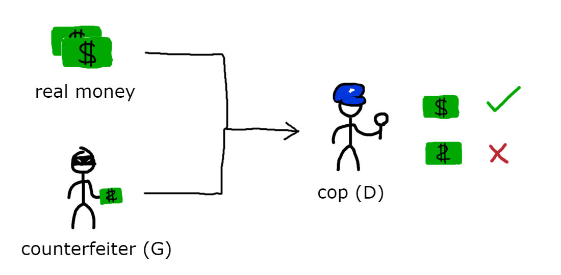
In practice the game is played by alternating stochastic gradient steps: k ascent steps on the discriminator, then one descent step on the generator. Writing the second expectation over x = G(z),
V(D, G) = \int_{\mathcal{X}} \Big( p_r(x) \log D(x) + p_g(x) \log\left(1 - D(x)\right) \Big) \, dx . \tag{2.2}
Writing p_g presumes P_g has a Lebesgue density, and Section 2.4 argues the opposite: P_g lives on a d_z-dimensional set with d_z \ll d, so no such density exists in exactly the regime we are about to analyse. Nothing below actually needs one. Take any measure \rho dominating both — the mixture P_r + P_g always does — and read p_r, p_g as the Radon–Nikodym derivatives dP_r/d\rho, dP_g/d\rho, with dx replaced by d\rho. Every step through Equation 2.3 goes through unchanged, because each is pointwise in the pair (p_r, p_g). It is the density notation that fails on disjoint supports, not the argument.
2.3.2 The optimal discriminator
Proposition 2.1 (Optimal discriminator) For a fixed generator, the discriminator that maximises Equation 2.2 is D^*_G(x) = \frac{p_r(x)}{p_r(x) + p_g(x)} on the set where p_r(x) + p_g(x) > 0.
Proof. The integrand depends on D only through y = D(x) at the same point, so we maximise pointwise. For a = p_r(x) \ge 0 and b = p_g(x) \ge 0, not both zero, let h(y) = a \log y + b \log(1 - y) on (0, 1). Then h'(y) = \frac{a}{y} - \frac{b}{1 - y}, \qquad h''(y) = -\frac{a}{y^2} - \frac{b}{(1-y)^2} < 0 , so h is strictly concave and its stationary point y = a/(a+b) is the maximiser. (If b = 0 the supremum is approached as y \to 1 but not attained — a first hint that disjoint supports cause trouble.)
The assumption doing the work is that D ranges over all functions. A neural discriminator can only approximate D^*_G.
2.3.3 What the generator minimises
Substitute D^*_G into V and write m = \frac{1}{2}(p_r + p_g) for the mixture. Since \frac{p_r}{p_r + p_g} = \frac{1}{2} \cdot \frac{p_r}{m},
\begin{aligned} C(G) := \max_D V(D, G) &= \mathbb{E}_{p_r}\left[\log \frac{p_r}{p_r + p_g}\right] + \mathbb{E}_{p_g}\left[\log \frac{p_g}{p_r + p_g}\right] \\ &= \mathbb{E}_{p_r}\left[\log \frac{p_r}{m}\right] - \log 2 + \mathbb{E}_{p_g}\left[\log \frac{p_g}{m}\right] - \log 2 \\ &= \mathrm{KL}(p_r \,\Vert\, m) + \mathrm{KL}(p_g \,\Vert\, m) - \log 4 = 2\,\mathrm{JSD}(p_r, p_g) - \log 4 . \end{aligned} \tag{2.3}
Theorem 2.1 (Global optimum of the GAN game) C(G) \ge -\log 4, with equality if and only if p_g = p_r. At that point D^*_G \equiv 1/2.
Proof. \mathrm{JSD} \ge 0 with equality iff p_r = p_g, since each KL term is zero iff its argument equals m. Plug into Equation 2.3; when p_g = p_r, Proposition 2.1 gives D^* = 1/2.
So in the idealised setting the game has the right fixed point. The rest of the lecture is about why reaching it is hard.
2.4 Why the JSD saturates on disjoint supports
2.4.1 The JSD is constant when supports do not overlap
Suppose P_r and P_g are concentrated on disjoint sets S_r and S_g. On S_r we have p_g = 0, so p_r / m = 2; on S_g, p_g / m = 2. Hence
\mathrm{KL}(p_r \Vert m) = \mathrm{KL}(p_g \Vert m) = \log 2, \qquad \mathrm{JSD}(p_r, p_g) = \log 2 ,
and C(G) = 2 \log 2 - \log 4 = 0, however far apart the two sets are. A generator one pixel away from the data and one producing pure noise get the same value, and the gradient of C with respect to \theta is zero.
This is the typical case, not a corner case (Arjovsky and Bottou 2017). Natural images concentrate near a low-dimensional manifold in \mathbb{R}^d, and the generator maps \mathbb{R}^{d_z} into \mathbb{R}^d with d_z \ll d, so P_g also lives on a low-dimensional set. Two such sets in general position intersect in a set of measure zero, and then a perfect discriminator exists: D = 1 on S_r, D = 0 on S_g.
2.4.2 What this does to the generator’s gradient
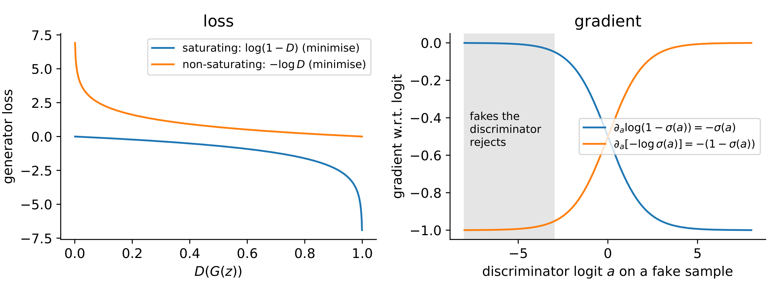
Write the discriminator as D = \sigma(a), where a(x) is the logit. By the chain rule the generator’s term in Equation 2.1 has gradient
\nabla_\theta \log\left(1 - \sigma(a)\right) = \frac{\partial \log(1 - \sigma(a))}{\partial a} \, \nabla_\theta a = -D(G_\theta(z)) \, \nabla_\theta a(G_\theta(z)). \tag{2.4}
When the discriminator confidently rejects the fakes, D(G(z)) \to 0 and the factor -D(G(z)) kills the gradient, however informative \nabla_\theta a is. The better the discriminator, the less the generator learns; Arjovsky and Bottou show that the generator gradient goes to zero as D approaches a perfect discriminator [2, Thm. 2.4]. Training therefore has a narrow window: too little discriminator training gives a wrong signal, too much gives none.
2.5 The non-saturating loss
2.5.1 The heuristic
Goodfellow et al. already proposed a fix (Goodfellow et al. 2014): instead of minimising \mathbb{E}_z[\log(1 - D(G(z)))], the generator minimises
\mathcal{L}_G^{\mathrm{NS}} = -\,\mathbb{E}_{z \sim p_z}\left[\log D(G(z))\right]. \tag{2.5}
Both losses push D(G(z)) upwards and share the fixed point p_g = p_r, but their gradients differ. With D = \sigma(a),
\frac{\partial}{\partial a}\left[-\log \sigma(a)\right] = -\left(1 - \sigma(a)\right) \longrightarrow -1 \quad \text{as } D \to 0 ,
so the fakes the discriminator rejects most confidently now receive the largest gradient instead of the smallest (Figure 2.2).
2.5.2 What the non-saturating loss actually minimises
The non-saturating loss is no longer the minimax game, so which divergence does it follow? Hold the discriminator at its optimum D^* for the current generator \theta_0 and differentiate with respect to \theta at \theta_0, treating D^* as fixed. Two identities do the work:
\log D^* - \log(1 - D^*) = \log \frac{p_r}{p_g} \quad\Longrightarrow\quad -\log D^* = \log \frac{p_g}{p_r} - \log(1 - D^*) ,
and, from Equation 2.3, \mathbb{E}_{p_r}[\log D^*] + \mathbb{E}_{p_g}[\log(1-D^*)] = 2\,\mathrm{JSD} - \log 4, where the first expectation does not depend on \theta. Taking \mathbb{E}_{p_g} of the first identity and differentiating gives [2, Thm. 2.5]
\nabla_\theta \, \mathbb{E}_{z}\left[-\log D^*(G_\theta(z))\right] = \nabla_\theta \left[ \mathrm{KL}(p_g \Vert p_r) - 2\,\mathrm{JSD}(p_r, p_g) \right]. \tag{2.6}
Two remarks. The -2\,\mathrm{JSD} term has the wrong sign: it pushes the distributions apart. And \mathrm{KL}(p_g \Vert p_r) is the reverse KL: it is infinite if the generator puts mass where there is no data, but costs almost nothing if the generator ignores part of the data. The non-saturating loss buys stable gradients at the price of a bias towards dropping modes.
2.6 Mode collapse
Mode collapse is when the generator covers only a few modes of the data even though each sample may look realistic — for example, one or two of eight Gaussians on a circle, or near-duplicate faces in a batch. A dynamic variant is mode hopping: the generator jumps from mode to mode as the discriminator learns to reject the current one.
Three parts of the objective invite it.
- The generator’s inner problem. For a fixed discriminator, the generator objective \mathbb{E}_z[-\log D(G(z))] is minimised by mapping every z to a single point \arg\max_x D(x). Theorem 2.1 is about \min_G \max_D, where the discriminator responds to the generator; alternating gradient steps are closer to alternating best responses, and the generator’s best response to a fixed D is a point mass.
- The divergence being followed. By Equation 2.6 the non-saturating loss follows the reverse KL, which is mode-seeking: missing a mode is cheap, inventing mass off the data is expensive.
- Per-sample judgement. The discriminator scores samples one at a time, so it cannot notice that a whole batch is the same image.
Remedies include minibatch discrimination (Salimans et al. 2016), unrolled GANs (Metz et al. 2017), and the IPM-based GANs below, whose gradient does not vanish when the discriminator is strong. What the first two actually compute, and how collapse is diagnosed, is in Section 2.18.3.
2.7 f-divergences and f-GAN
2.7.1 f-divergences
Definition 2.1 (f-divergence) Let f : (0, \infty) \to \mathbb{R} be convex and lower semicontinuous with f(1) = 0. For distributions P \ll Q with densities p, q, D_f(P \Vert Q) = \int_{\mathcal{X}} q(x) \, f\!\left(\frac{p(x)}{q(x)}\right) dx .
By Jensen’s inequality, D_f(P \Vert Q) \ge f\left(\int q \cdot \frac{p}{q}\right) = f(1) = 0. Different choices of f give familiar divergences (Table 2.1).
| Divergence | f(u) | f^*(t) | \operatorname{dom} f^* | g_f(v) | f^*(g_f(v)) |
|---|---|---|---|---|---|
| KL | u \log u | e^{t-1} | \mathbb{R} | v | e^{v-1} |
| Reverse KL | -\log u | -1 - \log(-t) | t < 0 | -e^{-v} | -1 + v |
| Pearson \chi^2 | (u - 1)^2 | t + t^2/4 | \mathbb{R} | v | v + v^2/4 |
| Squared Hellinger | (\sqrt{u} - 1)^2 | t / (1 - t) | t < 1 | 1 - e^{-v} | e^{v} - 1 |
| Jensen–Shannon | u \log u - (u+1)\log\frac{u+1}{2} | -\log(2 - e^{t}) | t < \log 2 | \log 2 - \log(1 + e^{-v}) | -\log\bigl(2 - 2\sigma(v)\bigr) |
| GAN | u \log u - (u+1)\log(u+1) | -\log(1 - e^{t}) | t < 0 | -\log(1 + e^{-v}) | -\log\bigl(1 - \sigma(v)\bigr) |
2.7.2 The Fenchel conjugate and the variational lower bound
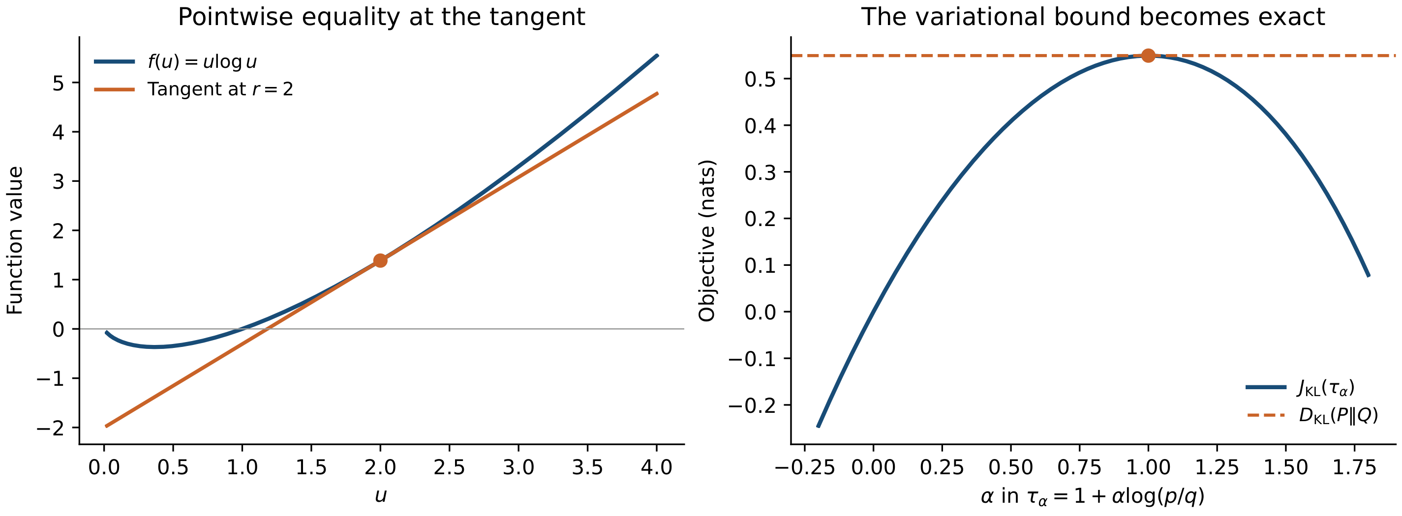
The Fenchel conjugate of f is f^*(t) = \sup_{u} \{ut - f(u)\}. For convex lower semicontinuous f the Fenchel-Moreau theorem gives f^{**} = f:
f(u) = \sup_{t \in \mathrm{dom} f^*} \{ tu - f^*(t) \}. \tag{2.7}
To compute a conjugate, solve f'(u) = t for u and substitute. For the GAN row: f'(u) = \log\frac{2u}{u+1} = t, which requires e^{t} < 2 and gives u = e^{t}/(2 - e^{t}). At this u the generator is f(u) = ut - \log\frac{u+1}{2}, so f^*(t) = ut - f(u) = \log\frac{u+1}{2} = -\log(2 - e^{t}). For Pearson, 2(u-1) = t gives u = 1 + t/2 and f^*(t) = t + t^2/4.
Now insert Equation 2.7 into Definition 2.1, choosing t = T(x) separately at each point:
\begin{aligned} D_f(P \Vert Q) &= \int q(x) \sup_{t} \left\{ t \, \frac{p(x)}{q(x)} - f^*(t) \right\} dx \\ &\ge \sup_{T \in \mathcal{T}} \Big( \mathbb{E}_{x \sim P}[T(x)] - \mathbb{E}_{x \sim Q}[f^*(T(x))] \Big). \end{aligned} \tag{2.8}
The inequality comes only from restricting T to a class \mathcal{T} (a neural network family); over all measurable T it is an equality (Nguyen et al. 2010), attained at T^*(x) = f'(p(x)/q(x)), where the supremum in Equation 2.7 is reached. The right-hand side involves only expectations, so it can be estimated from samples without knowing either density. That is what makes it usable for a GAN.
2.7.3 f-GAN as the general recipe
Nowozin, Cseke and Tomioka (Nowozin et al. 2016) take P = P_r, Q = P_\theta and turn Equation 2.8 into a game:
\min_\theta \max_\omega \; F(\theta, \omega) = \mathbb{E}_{x \sim P_r}\left[g_f(V_\omega(x))\right] - \mathbb{E}_{x \sim P_\theta}\left[f^*\!\left(g_f(V_\omega(x))\right)\right], \tag{2.9}
where V_\omega is an unconstrained network and g_f is an output activation mapping \mathbb{R} into the domain of f^* (for KL and Pearson, g_f(v) = v; for reverse KL, g_f(v) = -e^{-v}).
The original GAN, via the normalised generator. Taking the Jensen–Shannon row of Table 2.1, its conjugate needs t < \log 2, so take g_f(v) = \log 2 + \log \sigma(v) = \log\big(2\sigma(v)\big). Writing D(x) = \sigma(V_\omega(x)) gives T = \log(2D) and f^*(T) = -\log(2 - 2D) = -\log 2 - \log(1 - D), so
F(\theta, \omega) = \mathbb{E}_{P_r}[\log D(x)] + \mathbb{E}_{P_\theta}[\log(1 - D(x))] + \log 4 = V(D, G) + \log 4 ,
which is Equation 2.1 shifted by a constant — and it is the same constant that Equation 2.3 carries, since D_{f_{\mathrm{GAN}}} = 2\,\mathrm{JSD} = C(G) + \log 4. Maximising over \omega and minimising over \theta is therefore the same problem as Equation 2.1.
A word on that constant, because it is why Table 2.1 carries two rows that look like the same thing. The GAN row uses u \log u - (u+1)\log(u+1), which is what the f-GAN paper and the lecture both use (Ye 2026, 56–59), and it reproduces Equation 2.1 on the nose: g_f(v) = -\log(1+e^{-v}) gives f^*(g_f(v)) = -\log(1 - \sigma(v)), and the variational objective is exactly \mathbb{E}_{P_r}[\log D] + \mathbb{E}_{P_\theta}[\log(1-D)] with D = \sigma(V_\omega), with no constant to carry. That is its convenience and it is the reason to prefer it when deriving the original GAN.
What it is not is an f-divergence in the sense of Definition 2.1, because f(1) = -\log 4 \ne 0. The Jensen argument above does not apply to it, and the quantity it generates is 2\,\mathrm{JSD} - \log 4, which is negative whenever the two distributions are close. A reader who takes Definition 2.1 seriously would conclude that the GAN divergence is non-negative, and it is not. The Jensen–Shannon row is the same generator normalised so that f(1) = 0; it costs the \log 4 and buys back non-negativity. This is the same normalisation clash as the factor of two in Proposition 1.4 of the previous chapter, and the honest thing is to carry both and say which one is being used.
So the original GAN is not special: any f-divergence gives a GAN. The price is that every f-divergence depends only on the density ratio, so it cannot see how far apart two disjoint supports are, and the saturation problem is not solved within this family. How Equation 2.9 is optimised in practice, and what changes when f changes, is in Section 2.18.1.
2.8 LS-GAN and the Pearson chi-squared divergence
2.8.1 The least-squares objective
Mao et al. (Mao et al. 2017) replace the log loss by squared error against target labels a (fake), b (real) and c (what the generator wants the discriminator to say about its samples):
\begin{aligned} \min_D \; & \tfrac{1}{2}\,\mathbb{E}_{x \sim p_r}\left[(D(x) - b)^2\right] + \tfrac{1}{2}\,\mathbb{E}_{z \sim p_z}\left[(D(G(z)) - a)^2\right], \\ \min_G \; & \tfrac{1}{2}\,\mathbb{E}_{z \sim p_z}\left[(D(G(z)) - c)^2\right]. \end{aligned} \tag{2.10}
Here D has a linear output. With the sigmoid cross-entropy loss, a fake sample already on the “real” side of the decision boundary gives almost no gradient even if it is far from the data. The squared loss keeps penalising it in proportion to its distance from the target, so gradients do not vanish.
2.8.2 The optimal discriminator and the divergence
Pointwise, D minimises p_r(x)(D - b)^2 + p_g(x)(D - a)^2, a convex quadratic whose minimiser is
D^*(x) = \frac{b\,p_r(x) + a\,p_g(x)}{p_r(x) + p_g(x)} .
Add to the generator objective the term \tfrac{1}{2}\mathbb{E}_{p_r}[(D(x) - c)^2], which does not depend on G. With D = D^*,
2\,C(G) = \int \left(p_r + p_g\right)\left(D^* - c\right)^2 dx = \int \frac{\left((b - c)\,p_r + (a - c)\,p_g\right)^2}{p_r + p_g}\, dx .
Choose the labels so that b - c = 1 and b - a = 2 (hence a - c = -1), e.g. a = -1, b = 1, c = 0. The numerator becomes (p_r - p_g)^2 = \big(2p_g - (p_r + p_g)\big)^2 and
2\,C(G) = \int \frac{\big(2 p_g(x) - (p_r(x) + p_g(x))\big)^2}{p_r(x) + p_g(x)}\, dx = \chi^2_{\mathrm{Pearson}}\big(2 p_g \,\Vert\, p_r + p_g\big), \tag{2.11}
with \chi^2_{\mathrm{Pearson}}(P \Vert Q) = \int (p - q)^2 / q, the f-divergence with f(u) = (u-1)^2. It is zero iff p_g = p_r. (Mao et al. write the arguments in the opposite order; the integral is the same.) The popular choice a = 0, b = c = 1 does not satisfy the two conditions but behaves similarly in practice (Mao et al. 2017). LS-GAN therefore minimises a Pearson \chi^2-type divergence, which places it in the f-divergence family.
2.9 DCGAN: the architecture that made it train
Everything so far has been about the objective. None of it says what G and D should be, and for the first two years after Equation 2.1 that was the binding constraint: the objective was right and the models would not converge. DCGAN (Radford et al. 2016) is the paper that settled the architecture, and it is worth a section because every model in the rest of this chapter and the next is built on it.
2.9.1 The generator
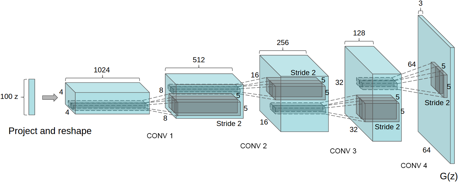
Figure 2.4 is the whole design. Spatial resolution doubles at each step while the channel count halves, so the tensor is reshaped from deep and small to shallow and large by learned upsampling rather than by interpolation.
2.9.2 Five rules
The paper’s contribution is not one architecture but a set of constraints that made the family trainable (Radford et al. 2016):
- Replace pooling with strided convolutions in the discriminator and fractionally-strided convolutions in the generator, so the network learns its own downsampling and upsampling.
- Use batch normalisation in both networks.
- Remove fully connected hidden layers in deeper architectures.
- In the generator use ReLU everywhere except the output, which uses tanh.
- In the discriminator use LeakyReLU everywhere.
Rules 1 and 3 are the same idea twice: take out the layers that do not respect spatial structure. Rule 2 is the one that interacts with the theory of this chapter. Batch normalisation keeps activations in a range where the discriminator’s gradient is informative, which attacks the saturation of Section 2.4 from the architecture side rather than from the loss side — the non-saturating loss of Section 2.5 and the Wasserstein critic of Section 2.11 are the two loss-side attacks on the same problem. Rules 4 and 5 are of a piece with it: a generator ReLU can output zero gradient on a whole half-space, and in the discriminator, where the gradient is the signal passed back to G, the leak is what keeps it alive.
Not every rule survived. Batch normalisation in the discriminator is now usually replaced, because it couples the examples in a minibatch and the gradient penalty of Section 2.12.2 is defined per example; the usual substitutes are layer or instance normalisation, which Section 3.3 of the next chapter treats properly.
2.9.3 What the latent space turned out to be
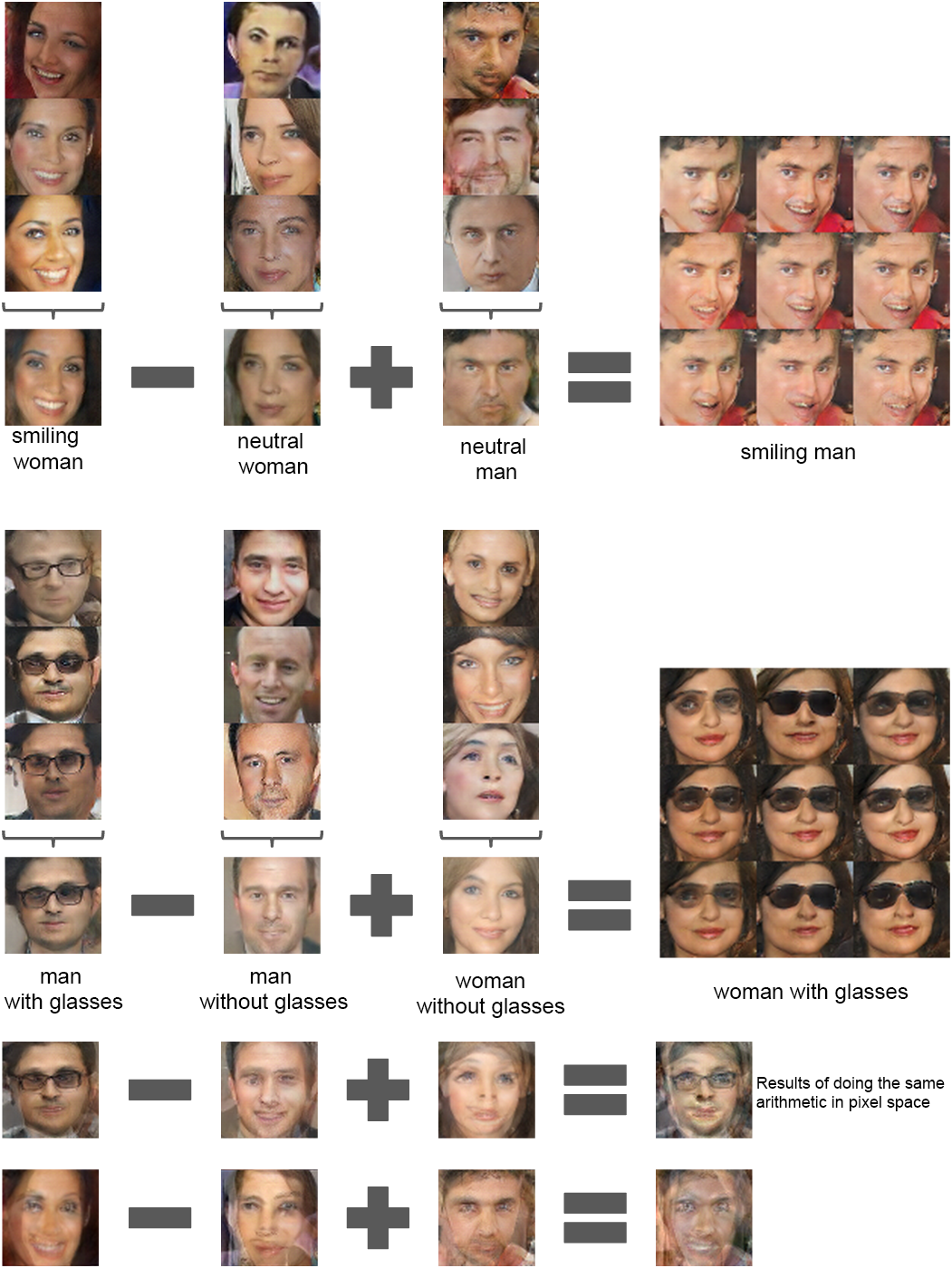
The result in Figure 2.5 was not designed for and is the reason DCGAN is remembered. Averaging the z vectors of smiling women, subtracting the average for neutral women, adding the average for neutral men, and decoding gives smiling men. Nothing in Equation 2.1 asks for this: the objective constrains the push-forward \mu_\theta = G_{\theta\#}\nu as a distribution and says nothing about how G_\theta arranges the latent space internally.
The bottom rows are the control, and they are what makes the claim non-trivial. The same arithmetic in pixel space gives ghosted overlays, because pixels have no such structure. So the linear structure is something the generator built, not something the data has.
This is the first appearance of a question the next two chapters are about. If directions in z carry meaning, can they be made to carry chosen meanings? InfoGAN below answers by adding a term that rewards it; Section 3.6 in the next chapter answers by changing where the latent code enters the network; and the \beta-VAE of Section 4.6 answers by pricing the information the code may carry.
2.10 InfoGAN
2.10.1 The mutual information term
A standard GAN is free to use its latent vector in an entangled way. InfoGAN (Chen et al. 2016) splits the input into noise z and a latent code c with a known, factored prior (for MNIST: one 10-way categorical code and two continuous codes, uniform on [-1, 1]), and asks that the code be recoverable from the output:
\min_G \max_D \; V(D, G) - \lambda\, I\big(c;\, G(z, c)\big). \tag{2.12}
2.10.2 The variational lower bound
I(c; x) = H(c) - H(c \mid x) needs the posterior P(c \mid x), which is intractable. Introduce an auxiliary distribution Q(c \mid x):
\begin{aligned} -H(c \mid x) &= \mathbb{E}_{x}\,\mathbb{E}_{c' \sim P(c \mid x)}\left[\log P(c' \mid x)\right] \\ &= \mathbb{E}_{x}\Big[ \mathrm{KL}\big(P(\cdot \mid x) \,\Vert\, Q(\cdot \mid x)\big) + \mathbb{E}_{c' \sim P(c \mid x)}\left[\log Q(c' \mid x)\right] \Big] \\ &\ge \mathbb{E}_{x}\,\mathbb{E}_{c' \sim P(c \mid x)}\left[\log Q(c' \mid x)\right], \end{aligned}
because the KL term is non-negative. The remaining expectation still samples from the posterior, but it does not have to: the pair (c', x) with x \sim P_G, c' \sim P(c \mid x) has the same joint law as (c, x) with c \sim p(c), x = G(z, c). Hence
I(c; G(z, c)) \;\ge\; L_I(G, Q) := \mathbb{E}_{c \sim p(c),\, z \sim p_z}\left[\log Q\big(c \mid G(z, c)\big)\right] + H(c), \tag{2.13}
which only needs samples from the prior. The bound is tight when Q equals the true posterior, and InfoGAN solves \min_{G, Q} \max_D V(D, G) - \lambda L_I(G, Q). Q is a small head on the discriminator’s convolutional trunk, so the extra cost is negligible; for a categorical code \log Q is a cross-entropy, for a continuous code a Gaussian Q gives a squared error.
2.10.3 What the codes actually disentangle
On MNIST the categorical code aligns with digit class (about 5% error as an unsupervised classifier) and the continuous codes with rotation and stroke width (Chen et al. 2016).
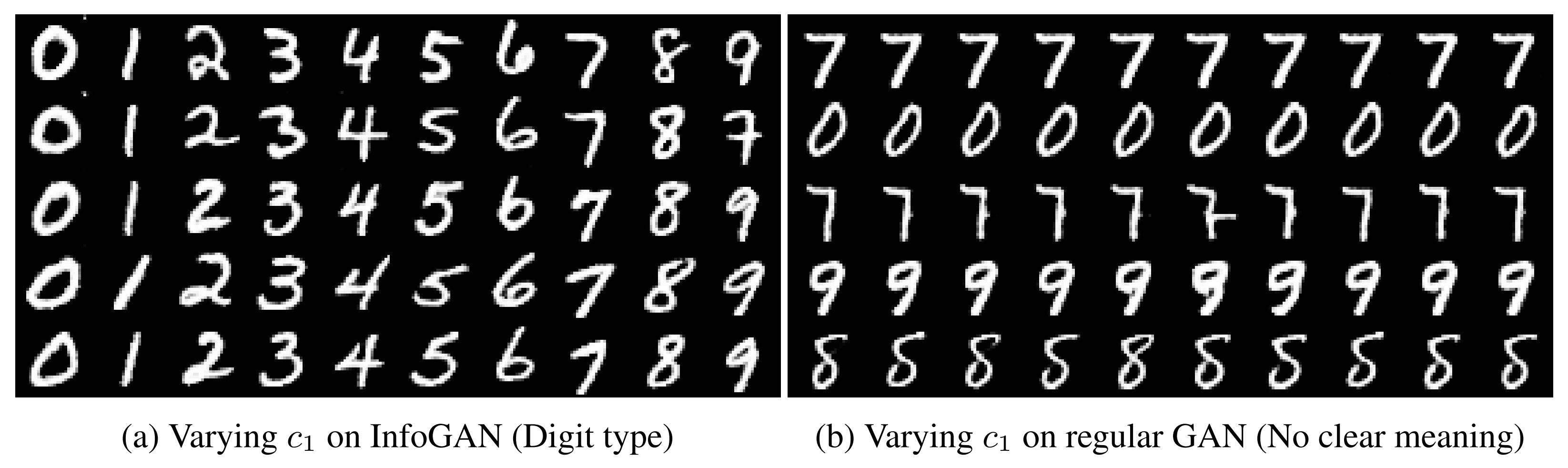
Mutual information is invariant under invertible reparametrisations of c, though, so the objective alone does not decide which factor a code captures; that comes from the prior, the architecture and the data. The other datasets, and how \lambda and the continuous-code head are set, are in Section 2.18.7.
2.11 W-GAN
2.11.1 The Wasserstein-1 distance
From the previous lecture, the Wasserstein-1 (earth mover’s) distance is
W_1(P, Q) = \inf_{\gamma \in \Pi(P, Q)} \mathbb{E}_{(x, y) \sim \gamma}\left[\Vert x - y \Vert\right], \tag{2.14}
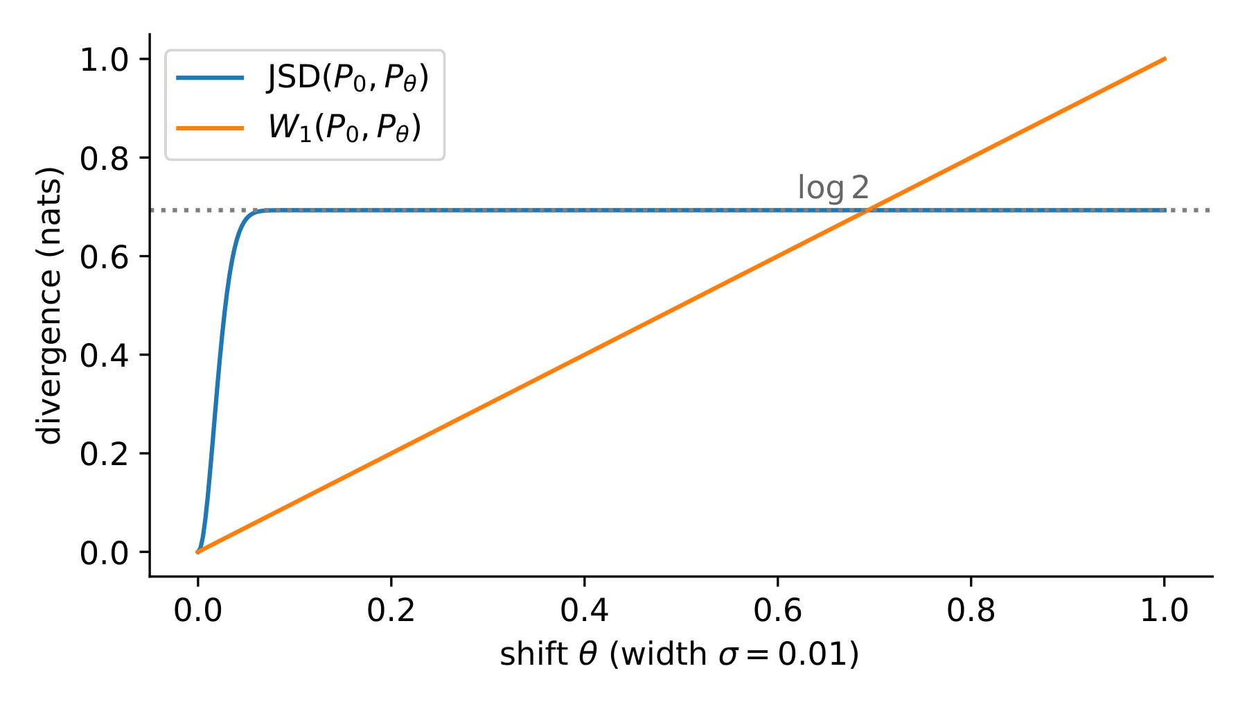
the cheapest cost of moving the mass of P onto Q. Unlike an f-divergence, it looks at where the mass is, not only at density ratios: on two disjoint supports W_1 grows with the gap while the JSD is stuck at \log 2 (see the worked example).
Theorem 2.2 (Continuity of W1 in the generator parameters) Let P_\theta be the law of G_\theta(z). If \mathbb{E}_z \Vert G_\theta(z) - G_{\theta'}(z) \Vert \to 0 as \theta' \to \theta, then \theta \mapsto W_1(P_r, P_\theta) is continuous. If moreover G_\theta is locally Lipschitz in \theta with an integrable constant, it is Lipschitz and hence differentiable almost everywhere [9, Thm. 1].
Proof. Using the same z for both generators defines a coupling of P_\theta and P_{\theta'}, so W_1(P_\theta, P_{\theta'}) \le \mathbb{E}_z \Vert G_\theta(z) - G_{\theta'}(z) \Vert. By the triangle inequality, \vert W_1(P_r, P_\theta) - W_1(P_r, P_{\theta'}) \vert \le W_1(P_\theta, P_{\theta'}) \to 0. Under the Lipschitz assumption the same bound is at most \mathbb{E}_z[L(\theta, z)]\,\Vert \theta - \theta' \Vert, and Rademacher’s theorem gives differentiability almost everywhere.
Neither statement holds for the JSD or the KL: in the worked example both jump at \theta = 0.
2.11.2 Kantorovich-Rubinstein duality
Equation 2.14 is an infimum over couplings, which we cannot optimise with samples. Its dual is a supremum over functions:
Theorem 2.3 (Kantorovich-Rubinstein duality) For P, Q with finite first moments, W_1(P, Q) = \sup_{\Vert f \Vert_L \le 1} \Big( \mathbb{E}_{x \sim P}[f(x)] - \mathbb{E}_{y \sim Q}[f(y)] \Big).
Proof. Weak duality. For any coupling \gamma and any 1-Lipschitz f, \mathbb{E}_P[f] - \mathbb{E}_Q[f] = \mathbb{E}_{(x, y) \sim \gamma}\left[f(x) - f(y)\right] \le \mathbb{E}_{\gamma}\left[\Vert x - y \Vert\right]. Take the sup over f on the left and the inf over \gamma on the right.
Why the dual has this form. The general Kantorovich dual is \sup \{ \mathbb{E}_P[\varphi] + \mathbb{E}_Q[\psi] : \varphi(x) + \psi(y) \le \Vert x - y \Vert \}. For a given \varphi the best \psi is the c-transform \varphi^c(y) = \inf_x [\Vert x - y \Vert - \varphi(x)], which is 1-Lipschitz. Replacing \varphi by \varphi^{cc} (also 1-Lipschitz) never lowers the objective, so we may take \varphi = u 1-Lipschitz. For such u, u^c(y) \le -u(y) (take x = y) and u^c(y) \ge -u(y) (since u(x) - u(y) \le \Vert x - y \Vert), so u^c = -u and the dual becomes \sup_{\Vert u \Vert_L \le 1} \mathbb{E}_P[u] - \mathbb{E}_Q[u]. Equality with the primal is Kantorovich duality [10, Thm. 5.10].
2.11.3 The W-GAN objective
Arjovsky, Chintala and Bottou (Arjovsky et al. 2017) parametrise f by a network f_w, the critic, constrained to be K-Lipschitz:
\min_\theta \max_{w : \Vert f_w \Vert_L \le K}\; \mathbb{E}_{x \sim P_r}[f_w(x)] - \mathbb{E}_{z \sim p_z}[f_w(G_\theta(z))]. \tag{2.15}
If the family is rich enough, the inner maximum is K \cdot W_1(P_r, P_\theta). There is no log and no sigmoid: the critic outputs a real score, not a probability. Under the assumptions of Theorem 2.2,
\nabla_\theta W_1(P_r, P_\theta) = -\,\mathbb{E}_{z \sim p_z}\left[\nabla_\theta f^{\mathrm{opt}}(G_\theta(z))\right],
where f^{\mathrm{opt}} is an optimal critic. This is the key difference from the original GAN. There, an optimal discriminator gives the gradient of a saturated JSD, which vanishes on disjoint supports (Equation 2.4). Here, an optimal critic gives exactly the gradient of W_1, which is informative everywhere. So the critic may, and should, be trained to optimality. In practice W-GAN runs 5 critic steps per generator step, and the authors report no mode collapse in their experiments.
2.12 Enforcing the Lipschitz constraint
Equation 2.15 needs \Vert f_w \Vert_L \le K, which a plain network does not satisfy. Three ways of enforcing it follow.
2.12.1 Weight clipping
The original W-GAN clips every weight to [-c, c] after each update, with c = 0.01. The parameter set is then compact, so every f_w is K-Lipschitz for some K. The authors call this “a clearly terrible way” to enforce the constraint (Arjovsky et al. 2017), and Gulrajani et al. (Gulrajani et al. 2017) document why:
- Capacity underuse. Most weights end up at \pm c, so the critic learns very simple functions.
- Exploding or vanishing gradients. Slightly too large a c explodes the gradient, slightly too small makes it vanish.
1 describes the evidence behind both.
2.12.2 WGAN-GP: the gradient penalty
The idea of (Gulrajani et al. 2017) starts from a property of the optimal critic.
Proposition 2.2 (Optimal critics have unit gradient on transport paths) Let f^{\mathrm{opt}} be an optimal critic and \gamma^* an optimal coupling. Then f^{\mathrm{opt}}(x) - f^{\mathrm{opt}}(y) = \Vert x - y \Vert for \gamma^*-almost every pair, and wherever f^{\mathrm{opt}} is differentiable at x_t = t x + (1 - t) y, \Vert \nabla f^{\mathrm{opt}}(x_t) \Vert = 1.
Proof. By strong duality \mathbb{E}_{\gamma^*}[\Vert x - y \Vert - (f^{\mathrm{opt}}(x) - f^{\mathrm{opt}}(y))] = 0, and the integrand is non-negative by the Lipschitz property, so it vanishes almost surely. A 1-Lipschitz function that rises by exactly \Vert x - y \Vert along a segment of that length must rise at unit rate throughout, so its directional derivative along (x - y)/\Vert x - y \Vert is 1; since the gradient norm is at most 1, it equals 1.
So instead of constraining weights, penalise the critic’s gradient norm where it matters, on points between real and generated samples:
L_{\mathrm{critic}} = \mathbb{E}_{\tilde{x} \sim P_\theta}\left[f_w(\tilde{x})\right] - \mathbb{E}_{x \sim P_r}\left[f_w(x)\right] + \lambda \, \mathbb{E}_{\hat{x}}\left[\left(\Vert \nabla_{\hat{x}} f_w(\hat{x}) \Vert_2 - 1\right)^2\right], \tag{2.16}
with \hat{x} = \epsilon x + (1 - \epsilon)\tilde{x}, \epsilon \sim U[0, 1], and \lambda = 10. The penalty is two-sided (it also pushes norms up to 1) and soft, and it is enforced only on the sampled lines, not everywhere. Because it is per-sample, the critic uses layer normalisation instead of batch normalisation.
2.12.3 Spectral normalisation
Miyato et al. (Miyato et al. 2018) bound the Lipschitz constant through the layers. For f = h_L \circ \cdots \circ h_1, \Vert f \Vert_L \le \prod_l \Vert h_l \Vert_L. A linear layer h(x) = Wx + b has \Vert h \Vert_L = \sigma_{\max}(W), the spectral norm, and ReLU is 1-Lipschitz. Normalising every weight matrix,
\bar{W} = \frac{W}{\sigma_{\max}(W)}, \tag{2.17}
therefore gives \Vert f \Vert_L \le 1. Instead of computing \sigma_{\max} exactly, one step of power iteration per update, with a persistent vector u, suffices because W changes slowly:
v \leftarrow \frac{W^\top u}{\Vert W^\top u \Vert_2}, \qquad u \leftarrow \frac{W v}{\Vert W v \Vert_2}, \qquad \sigma_{\max}(W) \approx u^\top W v .
Unlike clipping it keeps capacity, and unlike the gradient penalty it costs almost nothing. It is usually combined with the hinge loss of Geometric GAN. How tight the bound is, what is done for convolutional layers, and why the normalised layer behaves differently from a clipped one are in Section 2.18.5.
2.13 McGAN: mean and covariance feature matching
2.13.1 Integral probability metrics
W-GAN is one member of a larger family.
Definition 2.2 (Integral probability metric) For a class \mathcal{F} of real functions on \mathcal{X}, d_{\mathcal{F}}(P, Q) = \sup_{f \in \mathcal{F}} \Big\vert \mathbb{E}_P[f(x)] - \mathbb{E}_Q[f(x)] \Big\vert .
The 1-Lipschitz class gives W_1 (Theorem 2.3); \{\Vert f \Vert_\infty \le 1\} gives twice the total variation; the unit ball of a reproducing kernel Hilbert space gives the maximum mean discrepancy. IPMs compare expectations of test functions, so they involve no density ratios and stay finite and informative on disjoint supports.
2.13.2 Mean matching
Mroueh, Sercu and Goel (Mroueh et al. 2017) choose functions linear on top of a learned feature map \Phi_\omega : \mathcal{X} \to \mathbb{R}^m:
\mathcal{F}_{v, \omega} = \left\{ f(x) = \langle v, \Phi_\omega(x) \rangle \; : \; \Vert v \Vert_p \le 1 \right\}.
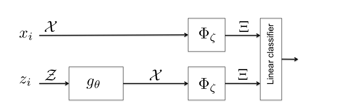
With \mu_\omega(P) = \mathbb{E}_{x \sim P}[\Phi_\omega(x)], linearity and the definition of the dual norm (1/p + 1/q = 1) give
d_{\mathcal{F}}(P, Q) = \sup_\omega \sup_{\Vert v \Vert_p \le 1} \langle v, \mu_\omega(P) - \mu_\omega(Q) \rangle = \sup_\omega \Vert \mu_\omega(P) - \mu_\omega(Q) \Vert_q . \tag{2.18}
The critic finds a feature space in which the two means differ most; the generator matches the means there (\Phi_\omega is kept bounded by clipping \omega).
A W-GAN critic whose last layer is linear, f(x) = \langle v, \Phi_\omega(x) \rangle, with v clipped to [-c, c], is exactly mean matching with p = \infty, i.e. the \ell_1 distance between feature means. The two are IPMs of the same form and differ only in the function class.
2.13.3 Covariance matching
Mean matching ignores second-order structure. McGAN adds f(x) = \langle u, \Phi_\omega(x) \rangle \langle v, \Phi_\omega(x) \rangle = u^\top \Phi_\omega(x) \Phi_\omega(x)^\top v for unit vectors u, v. With the uncentred covariance \Sigma_\omega(P) = \mathbb{E}_P[\Phi_\omega(x)\Phi_\omega(x)^\top],
\sup_{\Vert u \Vert = \Vert v \Vert = 1} u^\top \big(\Sigma_\omega(P) - \Sigma_\omega(Q)\big) v = \sigma_{\max}\big(\Sigma_\omega(P) - \Sigma_\omega(Q)\big), \tag{2.19}
the largest singular value of the difference. Using k orthonormal pairs instead gives the sum of the top k singular values. The generator then matches the leading directions of the feature covariance (Mroueh et al. 2017). Equation 2.18 and Equation 2.19 are what is being estimated, not what is coded; Section 2.18.2 writes the trained objective down.
2.14 Geometric GAN
2.14.1 The discriminator as a separating hyperplane
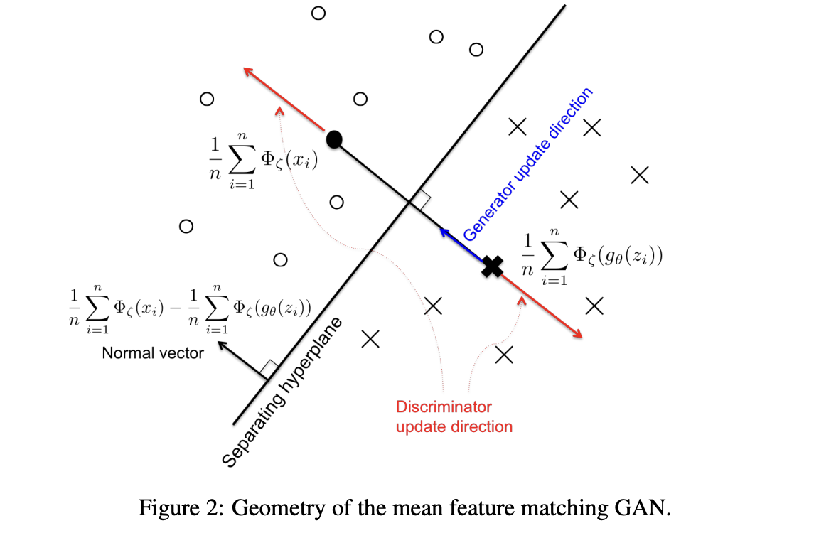
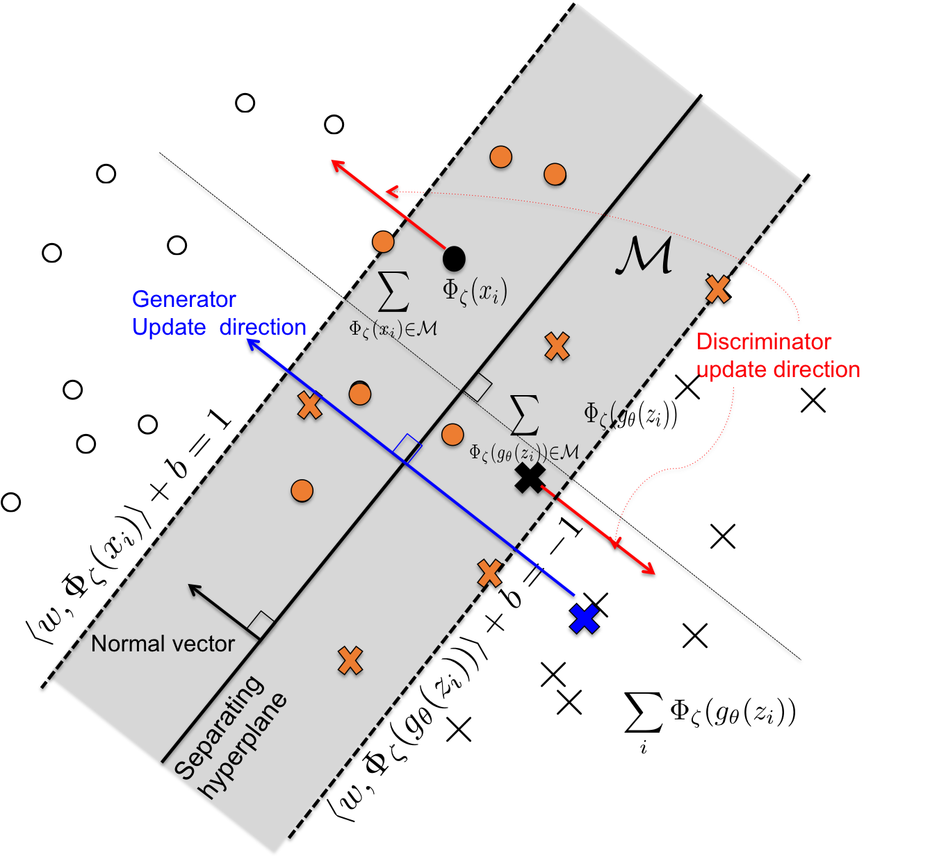
Lim and Ye (Lim and Ye 2017) also write the critic as linear in features, f(x) = \langle w, \Phi_\zeta(x) \rangle + b, and observe that separating real from fake features is a linear classification problem in feature space. The best-understood linear classifier is the support vector machine. The soft-margin SVM on real features (label +1) and fake features (label -1) solves
\min_{w, b} \; \frac{1}{2} \Vert w \Vert^2 + C \sum_i \max\big(0,\, 1 - f(x_i)\big) + C \sum_j \max\big(0,\, 1 + f(G(z_j))\big). \tag{2.20}
The hinge terms are zero for samples beyond the margin on their own side; only samples inside the margin or misclassified (the support vectors) contribute.
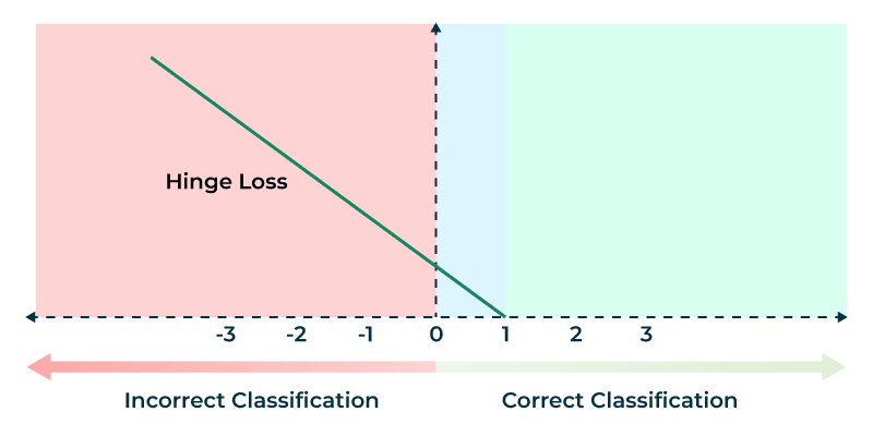
Dropping the \tfrac{1}{2}\Vert w \Vert^{2} term is not a normalisation identity, and it is worth being explicit about what replaces it: without a bound on \Vert w \Vert the hinge loss below can be driven down by rescaling w, and with it the margin interpretation. Lim and Ye instead fix the scale, taking \Vert w \Vert = 1 or constraining the trunk \Phi_\zeta — in practice by the spectral normalisation of Equation 2.17, which is why the two are almost always used together. Under that constraint the regulariser is a constant and the discriminator minimises the hinge loss
L_D = \mathbb{E}_{x \sim p_r}\left[\max\big(0, 1 - f(x)\big)\right] + \mathbb{E}_{z \sim p_z}\left[\max\big(0, 1 + f(G(z))\big)\right]. \tag{2.21}
2.14.2 What the generator does to the hyperplane
The decision boundary is the hyperplane \langle w, \phi \rangle + b = 0 in feature space, with normal vector w. The generator minimises L_G = -\mathbb{E}_{z}[f(G(z))], whose gradient with respect to a fake sample is \nabla_x f = J_{\Phi}(x)^\top w: the generator moves its features along the normal of the hyperplane, towards the real side. Training alternates between (i) fitting the maximum-margin hyperplane between real and fake features and (ii) pushing the fake features across it. By SVM duality, w = \sum_i \alpha_i \Phi(x_i) - \sum_j \beta_j \Phi(G(z_j)) with \alpha_i, \beta_j nonzero only on support vectors. Compare McGAN, whose direction \mu_\omega(P) - \mu_\omega(Q) averages all samples: Geometric GAN uses only the hard samples near the boundary. Lim and Ye analyse the equilibrium of the resulting game in (Lim and Ye 2017); Section 2.18.6 states what they prove and what it assumes.
2.14.3 Which distance the hinge discriminator estimates
Pointwise, the discriminator minimises p_r \max(0, 1 - t) + p_g \max(0, 1 + t) over t = f(x). This is piecewise linear with slope -p_r for t < -1, p_g - p_r on [-1, 1] and p_g for t > 1, so the minimum is at t = 1 if p_r > p_g and at t = -1 otherwise, with value 2\min(p_r, p_g). Using 2\min(a, b) = a + b - \vert a - b \vert,
\min_f L_D = \int 2\min\big(p_r, p_g\big)\, dx = 2 - \int \vert p_r - p_g \vert\, dx = 2\big(1 - \mathrm{TV}(p_r, p_g)\big).
So an unconstrained hinge discriminator measures the total variation distance. With a Lipschitz-constrained critic the loss behaves more like an IPM. The hinge loss with spectral normalisation became the default in later large-scale GANs.
2.15 What the critic’s loss does and does not tell you
Standard GAN. The discriminator is never optimal, and the JSD saturates anyway, so its loss is not a measure of sample quality: a falling generator loss can mean a better generator or a weaker discriminator.
W-GAN. If the critic is near-optimal and K-Lipschitz, the negative critic loss (without the penalty) estimates K \cdot W_1(P_r, P_\theta), which is continuous in \theta (Theorem 2.2). Arjovsky et al. show that it decreases steadily as samples improve and correlates with visual quality (Arjovsky et al. 2017), which makes it useful for debugging.
What it does not tell you.
- It is only a lower bound within the critic’s class. Arora et al. (Arora et al. 2017) show that a generator with small support can nearly fool a finite-capacity critic, so a small value does not certify diversity.
- Its scale is arbitrary. It depends on K — the clipping constant, \lambda or the architecture — so it cannot be compared across models or runs.
- It is not perceptual. W_1 with the Euclidean cost measures pixel distances, which do not match human judgement.
In practice samples are also compared with external metrics. The most common, the Frechet Inception Distance (Heusel et al. 2017), \mathrm{FID} = \Vert \mu_1 - \mu_2 \Vert_2^2 + \mathrm{Tr}\big(\Sigma_1 + \Sigma_2 - 2(\Sigma_1 \Sigma_2)^{1/2}\big), is the squared Wasserstein-2 distance between Gaussians fitted to Inception features: the same idea as McGAN, but with a fixed rather than learned feature map.
2.16 Worked example: JSD versus W1 on disjoint supports
Let P_0 and P_\theta be two narrow Gaussians of width \sigma = 0.01 centred at 0 (the data) and at \theta (a one-parameter generator). They approximate the point masses \delta_0 and \delta_\theta, whose supports are disjoint for \theta \ne 0. For the point masses everything can be computed by hand:
- \mathrm{JSD}(\delta_0, \delta_\theta) = \log 2 \approx 0.6931 for every \theta \ne 0, so C(G) = 2\,\mathrm{JSD} - \log 4 is 0 everywhere except at the optimum, where it jumps to -\log 4. Its derivative is zero wherever it exists.
- W_1(\delta_0, \delta_\theta) = \vert \theta \vert: the only coupling moves all the mass a distance \vert \theta \vert. Its derivative is \mathrm{sign}(\theta), so a gradient step on \theta always moves towards the data.
- An optimal critic is f^{\mathrm{opt}}(x) = -x\,\mathrm{sign}(\theta), whose gradient norm is 1 on the segment, as Proposition 2.2 says.
The code below checks this with the narrow Gaussians, using the fact that in one dimension W_1(P, Q) = \int \vert F_P(x) - F_Q(x) \vert\, dx for the cumulative distribution functions.
import numpy as np

def densities(theta, sigma, grid):
    p = np.exp(-0.5 * (grid / sigma) ** 2)
    q = np.exp(-0.5 * ((grid - theta) / sigma) ** 2)
    dx = grid[1] - grid[0]
    return p / (p.sum() * dx), q / (q.sum() * dx), dx

def jsd(p, q, dx):
    m = 0.5 * (p + q)
    kl = lambda a, b: np.sum(a[a > 0] * np.log(a[a > 0] / b[a > 0])) * dx
    return 0.5 * kl(p, m) + 0.5 * kl(q, m)

def w1(p, q, dx):
    # In one dimension W1 is the L1 distance between the two CDFs.
    return np.sum(np.abs(np.cumsum(p) - np.cumsum(q)) * dx) * dx

grid = np.linspace(-3.0, 5.0, 400001)
for theta in [0.0, 0.01, 0.02, 0.05, 0.1, 0.5, 1.0, 2.0]:
    p, q, dx = densities(theta, 0.01, grid)
    j = jsd(p, q, dx)
print(f"{theta:.2f} {j:.4f} {2 * j - np.log(4):.4f} {w1(p, q, dx):.4f}")| \theta | JSD | 2\,\mathrm{JSD} - \log 4 | W_1 |
|---|---|---|---|
| 0.00 | 0.0000 | -1.3863 | 0.0000 |
| 0.01 | 0.1114 | -1.1635 | 0.0100 |
| 0.02 | 0.3368 | -0.7126 | 0.0200 |
| 0.05 | 0.6759 | -0.0344 | 0.0500 |
| 0.10 | 0.6931 | 0.0000 | 0.1000 |
| 0.50 | 0.6931 | 0.0000 | 0.5000 |
| 1.00 | 0.6931 | 0.0000 | 1.0000 |
| 2.00 | 0.6931 | 0.0000 | 2.0000 |
Once the two bumps stop overlapping (from about \theta = 5\sigma = 0.05), the GAN value function is flat at 0: a generator at \theta = 0.1 and one at \theta = 2 are indistinguishable to it, and gradient descent has nothing to follow. W_1 equals \theta throughout and its gradient always points back to \theta = 0 (Figure 2.11). For a real image generator the “width” is zero in most directions of \mathbb{R}^d, so the flat regime is the normal one.
2.17 Connections and further reading
| Model | Distance (optimal discriminator) | Discriminator output |
|---|---|---|
| GAN (Goodfellow et al. 2014) | 2\,\mathrm{JSD} - \log 4 | probability, sigmoid |
| GAN, non-saturating (Goodfellow et al. 2014; Arjovsky and Bottou 2017) | follows \mathrm{KL}(p_g \Vert p_r) - 2\,\mathrm{JSD} | probability, sigmoid |
| f-GAN (Nowozin et al. 2016) | any D_f, via Equation 2.8 | g_f(V_\omega(x)) |
| LS-GAN (Mao et al. 2017) | Pearson \chi^2, Equation 2.11 | linear |
| W-GAN, WGAN-GP (Arjovsky et al. 2017; Gulrajani et al. 2017) | W_1, an IPM | linear, Lipschitz |
| McGAN (Mroueh et al. 2017) | IPM on feature means and covariances | linear in features |
| Geometric GAN (Lim and Ye 2017) | TV if unconstrained; SVM margin | linear, hinge loss |
The f-divergence family cannot see how far apart disjoint supports are; the IPM family can, at the cost of constraining the critic. This builds on the optimal transport of Lecture 01, and StyleGAN (Lecture 03) is trained with the non-saturating loss and a gradient penalty on real data.
2.18 Advanced topics
The chapter above follows the lecture. This section collects the material the lecture pointed at without developing: the algorithms behind three of the models, the evidence behind two claims about the Lipschitz constraint, and the equilibrium result for Geometric GAN. Each subsection is self-contained and none is needed to follow the main line.
2.18.1 The f-GAN algorithm in practice
Equation 2.9 is a saddle-point problem, and the obvious way to solve it — an inner loop maximising over \omega to convergence, then one step on \theta — is expensive and is not what Nowozin, Cseke and Tomioka do. Their single-step method takes one ascent step and one descent step per iteration,
\omega \leftarrow \omega + \eta \, \nabla_\omega F(\theta, \omega) , \qquad \theta \leftarrow \theta - \eta \, \nabla_\theta F(\theta, \omega) , \tag{2.22}
with both gradients taken at the same (\theta,\omega), so a single pass over a minibatch produces both. The justification is local. Near a saddle point (\theta^*, \omega^*) at which F is strongly concave in \omega and strongly convex in \theta, the iteration is a contraction for \eta small enough, and the authors give the resulting local geometric convergence rate. Neither hypothesis holds globally — GAN objectives are not convex-concave in the parameters — so this is an argument for why the scheme is stable once it is close, not a convergence proof.
Two practical points follow from the recipe rather than from the theory. The output activation g_f is not cosmetic: it is what keeps V_\omega inside \mathrm{dom}\, f^*, and choosing it badly makes f^*(g_f(V_\omega)) infinite on the first batch. And the choice of f is visible in the samples. Nowozin et al. report that models trained with different divergences from Table 2.1 differ noticeably at the same architecture and budget, in the direction the divergences predict: the mass-covering ones spread over the data and the mode-seeking ones sharpen. This is the same asymmetry as the reverse-KL bias of Equation 2.6, now selected deliberately rather than inherited by accident.
2.18.2 McGAN: the objective as it is trained
Equation 2.18 and Equation 2.19 identify what the mean- and covariance-matching IPMs equal; neither is what a program optimises. The trained problem is a minimax over the feature map and the projection directions together. For the mean term, with \Phi_\omega the feature map and \mu_\omega(P) = \mathbb{E}_P[\Phi_\omega],
\min_\theta \; \max_{\omega, \, \Vert v \Vert_2 \le 1} \; \big\langle v, \, \mu_\omega(P_r) - \mu_\omega(P_\theta) \big\rangle , \tag{2.23}
and for the covariance term, with U, V \in \mathbb{R}^{m \times k} ranging over matrices with orthonormal columns,
\min_\theta \; \max_{\omega, \, U^\top U = V^\top V = I_k} \; \operatorname{tr}\Big( U^\top \big( \Sigma_\omega(P_r) - \Sigma_\omega(P_\theta) \big) V \Big) \;=\; \min_\theta \max_\omega \; \sum_{i \le k} \sigma_i\big( \Sigma_\omega(P_r) - \Sigma_\omega(P_\theta) \big) , \tag{2.24}
the identity being the Ky Fan variational characterisation of the sum of the top k singular values. McGAN trains the sum of the two terms.
Three constraints have to be handled, and each is a line of code rather than a theorem.
- \Phi_\omega must be bounded, or the supremum over \omega diverges: a feature map free to scale up makes any non-zero difference of means arbitrarily large. McGAN clamps \omega to a box after each update, the same device, with the same drawbacks, as the weight clipping of
- U and V must stay orthonormal. They are points on a Stiefel manifold, and an unconstrained gradient step leaves it, so the step is followed by a retraction — in practice a QR or polar factorisation of the updated matrix, keeping the orthonormal factor.
- The two players alternate. Ascent on (\omega, U, V) and descent on \theta, in the same single-step style as Equation 2.22.
Written out this way the relationship to the rest of the chapter is plain. Mean matching with k = 0 and a clipped linear last layer is the W-GAN critic of Equation 2.15; replacing the learned \Phi_\omega by a fixed feature map and taking both terms gives the Frechet Inception Distance; and the whole family sits inside Definition 2.2, differing only in the class \mathcal{F}.
2.18.3 Mode collapse: what the standard remedies compute
The chapter names minibatch discrimination and unrolled GANs. Each repairs a different one of the three causes listed above.
Minibatch discrimination answers the third cause, that the discriminator judges samples one at a time. Salimans et al. give the discriminator a feature of the batch, not of the sample. Take the trunk’s features \phi(x_i) \in \mathbb{R}^A for the n samples in a batch, map each through a learned tensor T \in \mathbb{R}^{A \times B \times C} to a matrix M_i \in \mathbb{R}^{B \times C}, and give the discriminator the extra features
o(x_i)_b = \sum_{j \ne i} \exp\big( - \Vert M_{i,b} - M_{j,b} \Vert_1 \big) , \qquad b = 1, \dots, B , \tag{2.25}
concatenated to \phi(x_i). A batch of near-duplicates makes every o(x_i)_b large, and a diverse batch makes it small, so a collapsed generator is now detectable by a single discriminator evaluation. The discriminator is no longer a function of one sample, which is a real change to the game, but it is a change in exactly the direction the failure points.
Unrolled GANs answer the first cause, that the generator’s best response to a fixed discriminator is a point mass. Metz et al. let the generator see the discriminator’s reply: starting from the current \omega, unroll k discriminator ascent steps as a differentiable function \omega^{k}(\theta) and give the generator the loss F\big(\theta, \omega^{k}(\theta)\big), differentiating through the unrolled steps. The extra term \partial \omega^{k}/\partial \theta is what tells the generator that piling mass on one mode will be punished a few steps later. At k = 0 this is the ordinary alternating scheme; k of five to ten is enough to stop the rotation on the eight-Gaussians toy problem, at k times the memory and roughly k times the cost.
Diagnosis is mostly visual, and worth saying plainly because there is no scalar for it. The standard probe is a two-dimensional mixture — eight Gaussians on a circle, or a spiral — where the generator’s output can simply be plotted against the target over training: a collapsing generator shows as mass on a subset of the modes, and mode hopping as that subset moving. On images the cheap check is near-duplicate samples within a batch. The critic loss is not a diagnostic: 1 and the discussion of what the critic’s loss does not tell you both apply here, and Arora et al.’s point is precisely that a small critic value does not certify diversity.
2.18.4 What weight clipping does to the critic
The two failures the chapter asserts are both documented by Gulrajani et al., and the evidence is worth having because it explains why the gradient penalty is shaped the way it is.
Capacity. A histogram of the critic’s weights after training with clipping is bimodal, with almost all the mass at exactly \pm c. The clipped critic is therefore close to a sign pattern times c, and the functions it can express are correspondingly crude. On two-dimensional toy distributions the authors plot the value surfaces the critic learns: with clipping these are simple, low-order surfaces that ignore the finer structure of the data, while a gradient-penalised critic follows it. The point is not that the clipped critic is inaccurate by a little, but that it is solving a much smaller problem than the architecture allows.
Gradients. Clipping interacts badly with depth. The critic’s gradient scales roughly as a product of per-layer factors, each controlled by c, so the product is exponential in the number of layers: a c slightly too large makes it explode and slightly too small makes it vanish, with the usable window narrowing as the critic gets deeper. Batch normalisation hides this for a while, which is part of why the pathology took a year to be described.
Both observations point the same way: constrain the function, not the parameters. That is what Equation 2.16 does by penalising the gradient norm where Proposition 2.2 says it should be one, and what Equation 2.17 does by normalising each layer’s spectral norm.
2.18.5 Spectral normalisation: how tight is the bound?
Three caveats belong with Equation 2.17, none of which changes the conclusion that it works, but all of which change what it is claimed to do.
The bound is loose. \Vert f \Vert_L \le \prod_l \sigma_{\max}(W_l) holds with equality only if each layer’s top singular direction is aligned with the next layer’s, which is not what training produces. The true Lipschitz constant of a trained network is typically orders of magnitude below the product, so a spectrally normalised critic is not “1-Lipschitz and no less”: it satisfies the constraint with room to spare, and the effective constraint is harder to state than the nominal one.
Convolutions are approximated. \sigma_{\max} in Equation 2.17 is computed by reshaping the kernel W \in \mathbb{R}^{c_{\text{out}} \times c_{\text{in}} \times k \times k} to a c_{\text{out}} \times (c_{\text{in}}k^{2}) matrix and taking that matrix’s spectral norm. That is not the operator norm of the convolution, which depends on the input resolution, the stride and the padding, and can be larger. The implementation everyone uses is therefore an approximation to an already loose bound. It is a good approximation in practice, and the reason the discrepancy is tolerable is the looseness above.
Why it is not clipping. The interesting difference is in the gradient. Differentiating through \bar{W} = W / \sigma_{\max}(W) gives, for the loss V,
\frac{\partial V}{\partial W} = \frac{1}{\sigma_{\max}(W)} \left( \frac{\partial V}{\partial \bar{W}} - \Big\langle \frac{\partial V}{\partial \bar{W}}, \, \bar{W} \Big\rangle u_1 v_1^{\!\top} \right) , \tag{2.26}
where u_1, v_1 are the leading singular vectors. The update is the normalised gradient with its component along u_1 v_1^{\!\top} removed: whatever the loss would gain by growing the top singular value alone is subtracted out. Miyato et al. read this as a regulariser against the layer collapsing towards rank one. Clipping has no such term — it drives every entry to \pm c, which flattens the spectrum by force — and that is the mechanism behind the capacity difference of 1.
2.18.6 Geometric GAN: the equilibrium
The chapter derives the hinge loss and the direction the generator moves, and then defers. What Lim and Ye prove is a statement about the two clouds of features, \Phi_\zeta(x) for x \sim P_r and \Phi_\zeta(G_\theta(z)) for z \sim p_z.
At each round the discriminator step fits the maximum-margin hyperplane between the two clouds, and the generator step moves the fake features along its normal w towards the real side. Lim and Ye show that this pair of updates decreases the margin: the geometry of the SVM solution means the displacement is concentrated on the support vectors, which are exactly the fake features nearest the boundary, so the step removes the separation where it is smallest. Iterating, the two clouds converge to each other and the margin collapses; at the equilibrium no hyperplane separates them, which for a linear discriminator on those features is the statement that the two feature distributions coincide.
What the argument assumes is worth naming, because it is where the gap to practice sits. It treats the discriminator step as solving the SVM to optimality rather than taking one gradient step; it holds the feature map \Phi_\zeta fixed while the hyperplane and the generator move, so it is a statement about the geometry in a given feature space and not about learning that space; and it needs the scale fixed, the constraint discussed after Equation 2.20, since otherwise the margin can be changed by rescaling w without moving anything. Matching feature distributions is also weaker than matching the distributions themselves: it is exactly as strong as the feature map is discriminative, which is the same caveat that Definition 2.2 carries for every member of this family.
2.18.7 InfoGAN: what the codes capture
The chapter reports the MNIST result. The paper’s case rests on the other datasets, where the codes are less obviously the labels one would have supplied anyway.
| Dataset | Discrete code | Continuous codes |
|---|---|---|
| MNIST | digit class, about 5% error | rotation, stroke width |
| 3D faces | — | azimuth, elevation, lighting, width |
| 3D chairs | chair type | rotation, width |
| CelebA | presence of glasses, hairstyle | azimuth, emotion |
The evidence in each row is a latent traversal: fix z, sweep one code across its range, and look at the row of images. A code that has captured a factor produces a smooth, monotone change in that factor and leaves the rest alone. This is worth stating as the standard of evidence, because it is the only one available — there is no ground-truth factorisation to score against on CelebA, and the claim being made is about what a human sees in the traversal.
Two settings matter and neither is in Equation 2.12. The weight \lambda is not shared: the paper uses \lambda = 1 for discrete codes and a smaller value for continuous ones, because \log Q is a cross-entropy in the first case and a Gaussian log-density in the second, and the two are on different scales; too large a \lambda on a continuous code lets the information term dominate and the samples degrade. And for a continuous code the Gaussian head outputs both a mean and a variance, with the variance learned rather than fixed: a fixed variance makes \log Q a plain squared error, and the learned one lets the network express how confident the code is recoverable, which the paper found necessary for the continuous codes to separate.
Based on the scribe note of Sangyun Won, with material from Inhyeok Jeong and Hyungkwon Lee; edited by Jong Chul Ye.