1 Statistical Distance and Optimal Transport
1.1 Overview
A generative model does not produce a single number that we can compare against a label. It produces a whole distribution, and training it means making that distribution resemble the distribution the data came from. So before any architecture is discussed, we need an answer to a prior question: given two probability distributions over the same space, what does it mean to say that one is close to the other, and how close?
This lecture gives two answers, and they are genuinely different. The first compares distributions pointwise, through the ratio of their densities; this produces the family of f-divergences, of which the Kullback–Leibler and Jensen–Shannon divergences are the members that generative modelling actually uses. The second compares them by asking how much work it takes to carry the mass of one distribution onto the other; this produces optimal transport and the Wasserstein distances. The distinction is not decorative. We will see that when two distributions have disjoint supports — which, for a generative model of images, is the normal situation rather than an edge case — every f-divergence is constant and therefore carries no gradient, while the Wasserstein distance still varies smoothly. That single fact is the reason the GAN literature moved from the original minimax objective to the Wasserstein one, and it is the reason this material comes first in the course.
By the end the reader should be able to state and prove what an f-divergence is and when it is finite, derive the Kullback–Leibler and Jensen–Shannon divergences from their generators, recognise integral probability metrics as the dual-norm view of the same problem and estimate one of them from samples, set up both Monge’s and Kantorovich’s transport problems and say why the first can fail in three different ways, prove Kantorovich duality in the discrete case and read off from it both the Kantorovich–Rubinstein form of W_{1} and the c-cyclical monotonicity of optimal plans, and identify the optimal transport map between two Gaussians as an instance of Brenier’s theorem.
This chapter assumes the metric space, convexity and duality material of the preliminaries chapter and does not restate it.
1.2 Notation
| Symbol | Meaning |
|---|---|
| \mathcal{X}, \mathcal{Y} | Polish spaces; the data space and the latent space |
| \mathcal{P}(\mathcal{X}) | Borel probability measures on \mathcal{X} |
| \mu, \nu | probability measures; \mu is the source, \nu the target |
| P, Q | the same measures when densities or masses are meant |
| \nu \ll \mu | \nu is absolutely continuous with respect to \mu |
| d\nu / d\mu | Radon–Nikodym derivative of \nu with respect to \mu |
| T_{\#}\mu | push-forward of \mu under the map T |
| \Pi(\mu,\nu) | couplings of \mu and \nu |
| c(x,y) | transport cost from x to y |
| \varphi^{c} | c-transform of the potential \varphi |
| \mathrm{Lip}_{1}(\mathcal{X}) | 1-Lipschitz real functions on \mathcal{X} |
| G_{\theta} | generator with parameters \theta |
| p_{\text{data}} | the unknown data distribution |
Throughout, \log is the natural logarithm and the convention 0 \log 0 = 0 is in force, justified by continuity of t \log t at t = 0.
1.3 Why the distance between distributions is the question
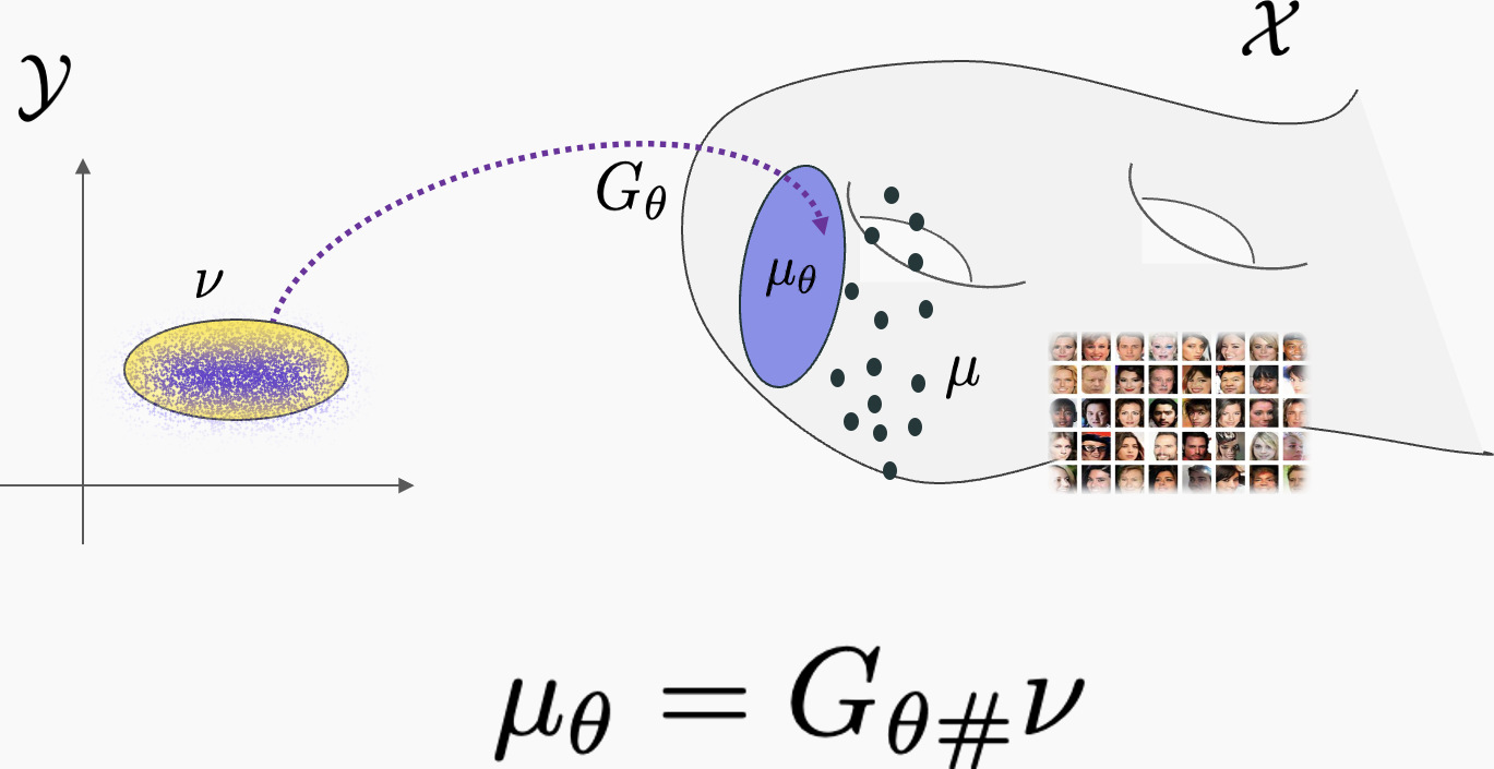
Fix a latent space \mathcal{Y} carrying a simple reference measure \nu — in practice \nu = \mathcal{N}(0, I) — and a data space \mathcal{X}. A generator is a measurable map G_{\theta} : \mathcal{Y} \to \mathcal{X}. It does not model a density directly. What it gives us is a procedure for drawing samples: take z \sim \nu and return G_{\theta}(z). The distribution of the result is the image of \nu under G_{\theta}, written
\mu_{\theta} = G_{\theta \#} \nu , \tag{1.1}
and made precise in Definition 1.2 below and drawn in Figure 1.1. Training the generator means choosing \theta so that \mu_{\theta} resembles p_{\text{data}}, which we only ever see through a finite sample. So we need a function D(\mu_{\theta}, p_{\text{data}}) that is small exactly when the two agree, and — this is the part that is easy to forget — whose gradient in \theta points somewhere useful when they do not.
Written out, the whole of generative modelling in this chapter is
\min_{\theta} \, D(\mu_{\theta}, \mu) \qquad \text{subject to} \qquad \mu_{\theta} = G_{\theta \#} \nu , \tag{1.2}
the form in which the lecture states it (Ye 2026, 51) and the one that organises the geometric reading of GANs due to Lei and co-authors (Lei et al. 2017). Everything that follows is a choice of D in Equation 1.2, and the chapter is in effect a catalogue of those choices and of what each one does to the gradient.
There is an obstruction, and it is structural rather than accidental. The support of \mu_{\theta} is contained in G_{\theta}(\mathcal{Y}), the image of a space of dimension \dim \mathcal{Y}, which in practice is a hundred or so. The data are believed to lie near a manifold of similarly low dimension inside a pixel space of dimension 10^{5} or more. Two such sets, both of measure zero in the ambient space, generically fail to overlap. Any discrepancy built out of the ratio of two densities is therefore being asked to compare 0/0 almost everywhere, and we will prove in Section 1.7 that it responds by saturating at a constant. Keeping that obstruction in view is what organises the rest of the chapter.
1.4 The measure-theoretic minimum
This section fixes three definitions that the rest of the chapter uses without further comment. It is deliberately brief; the preliminaries chapter treats measure and integration properly.
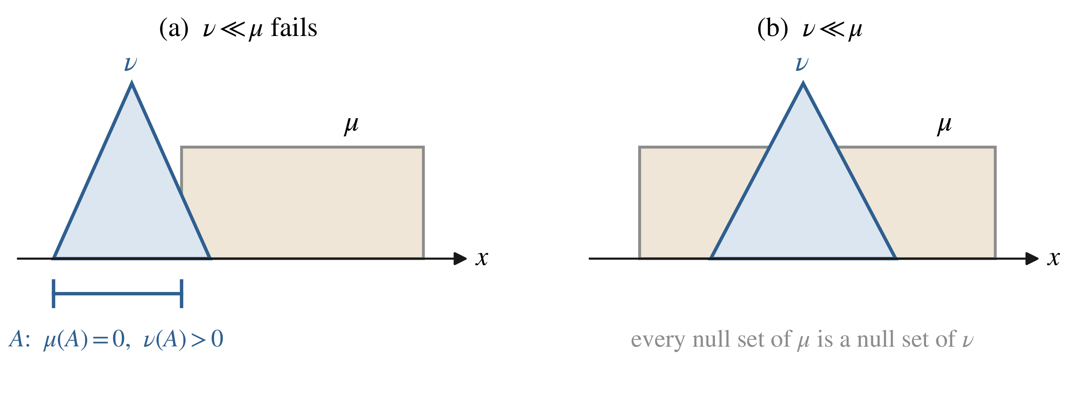
Definition 1.1 (Absolutely continuous measure) Let \mu and \nu be measures on a measurable space (\Omega, \mathcal{F}). We say \nu is absolutely continuous with respect to \mu, written \nu \ll \mu, if \mu(A) = 0 implies \nu(A) = 0 for every A \in \mathcal{F}.
The condition says that \nu cannot put mass where \mu puts none. It is the exact hypothesis under which a density of \nu with respect to \mu can exist, which is the content of the next theorem. Figure 1.2 contrasts the two cases.
Theorem 1.1 (Radon–Nikodym) Let \lambda and \nu be \sigma-finite measures on (\Omega, \mathcal{F}) with \lambda \ll \nu. Then there is a non-negative \mathcal{F}-measurable function g on \Omega, unique up to \nu-null sets, such that
\lambda(A) = \int_{A} g \, d\nu , \qquad A \in \mathcal{F} . \tag{1.3}
The function g is written d\lambda / d\nu. A proof is given in Section 1.16 rather than here, because the argument is self-contained but long enough to interrupt the development. An ordinary probability density function is the special case in which \nu is Lebesgue measure: writing p = dP/dx recovers P(A) = \int_{A} p(x) \, dx.
Definition 1.2 (Push-forward of a measure) Let (\mathcal{X}_{1}, \mathcal{B}_{1}) and (\mathcal{X}_{2}, \mathcal{B}_{2}) be measurable spaces, \mu a measure on the first, and T : \mathcal{X}_{1} \to \mathcal{X}_{2} measurable. The push-forward T_{\#}\mu is the measure on \mathcal{B}_{2} defined by
(T_{\#}\mu)(A) = \mu\bigl(T^{-1}(A)\bigr) = \mu\bigl(\{ x : T(x) \in A \}\bigr) . \tag{1.4}
Read Equation 1.4 as a statement about sampling: if x \sim \mu then T(x) \sim T_{\#}\mu. For a generator this is exactly Equation 1.1, and it is worth noting what the definition does not require. There is no inverse of T anywhere in it — only the preimage of a set, which exists for any map — and no density. A generator that collapses a whole region of latent space to one image is perfectly well described.
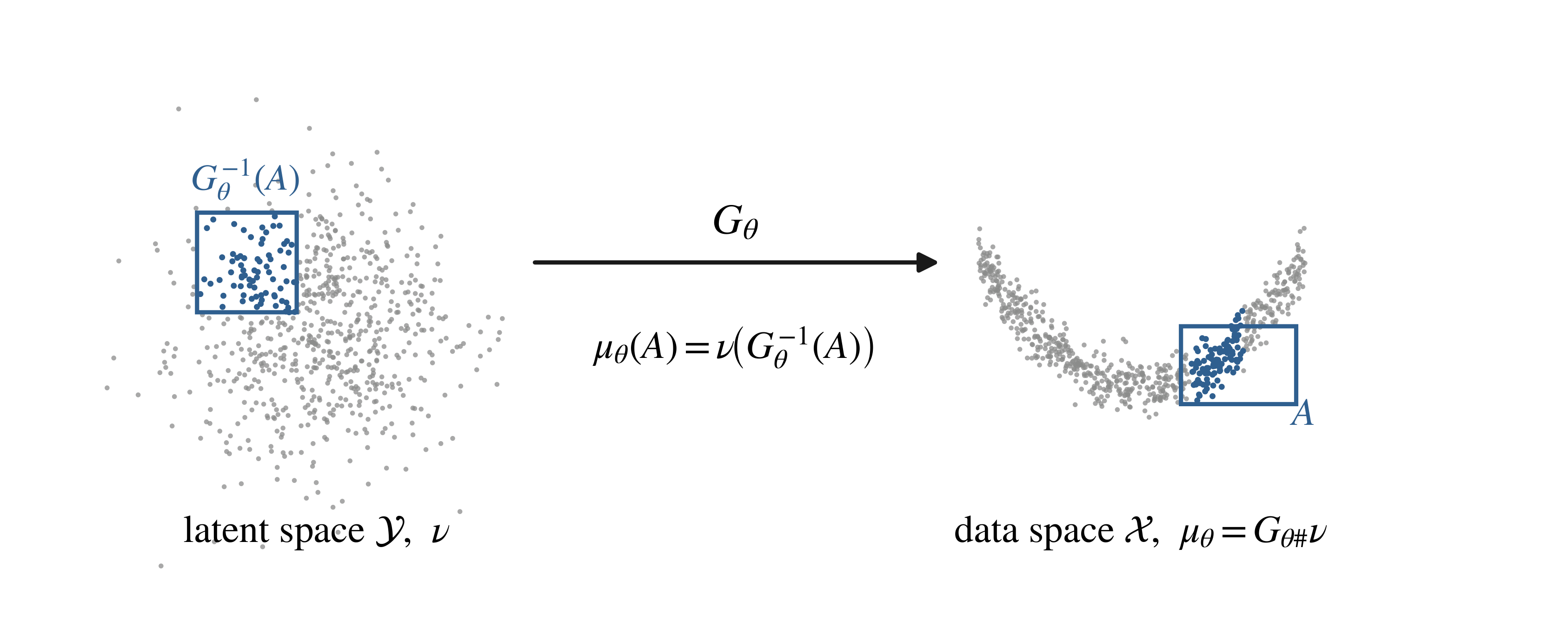
Figure 1.3 is Equation 1.4 with the sets drawn in.
The following lemma is used repeatedly and is never stated in the lecture, so we prove it.
Lemma 1.1 (Change of variables) Let T : \mathcal{X}_{1} \to \mathcal{X}_{2} be measurable and let h : \mathcal{X}_{2} \to [0, \infty] be measurable. Then
\int_{\mathcal{X}_{2}} h \, d(T_{\#}\mu) = \int_{\mathcal{X}_{1}} (h \circ T) \, d\mu . \tag{1.5}
Proof. Take first h = \mathbf{1}_{A} for A \in \mathcal{B}_{2}. The left-hand side is (T_{\#}\mu)(A), which is \mu(T^{-1}(A)) by Equation 1.4. The right-hand side is \int \mathbf{1}_{A}(T(x)) \, d\mu(x), and \mathbf{1}_{A}(T(x)) = \mathbf{1}_{T^{-1}(A)}(x), so it is also \mu(T^{-1}(A)). The two sides agree.
By linearity of the integral they agree for non-negative simple functions. For general measurable h \geq 0 choose simple h_{n} \uparrow h pointwise; then h_{n} \circ T \uparrow h \circ T pointwise, and monotone convergence applied on each side gives the result. An integrable h of arbitrary sign follows by splitting into h^{+} and h^{-}.
In particular, taking h to be a cost function turns an integral against a push-forward measure into an integral against the original one; this is the step that makes Monge’s problem in Section 1.10 computable at all.
1.5 Metrics and divergences are not the same thing
Definition 1.3 (Metric) A metric on a set \mathcal{X} is a function d : \mathcal{X} \times \mathcal{X} \to \mathbb{R}_{+} such that for all x, y, z \in \mathcal{X}:
- d(x,y) \geq 0;
- d(x,y) = 0 if and only if x = y;
- d(x,y) = d(y,x);
- d(x,z) \leq d(x,y) + d(y,z).
Definition 1.4 (Divergence) A divergence on \mathcal{P}(\mathcal{X}) is a function D : \mathcal{P}(\mathcal{X}) \times \mathcal{P}(\mathcal{X}) \to [0, \infty] satisfying only conditions 1 and 2 of Definition 1.3. Symmetry and the triangle inequality are not required.
The distinction is exactly what separates the two halves of this chapter. The f-divergences of Section 1.6 satisfy only the first two conditions: D_{\mathrm{KL}}(P \Vert Q) and D_{\mathrm{KL}}(Q \Vert P) are different numbers, and there is no triangle inequality relating three distributions. The Wasserstein distance of Section 1.9 satisfies all four and is a metric in the full sense — we prove this as Theorem 1.3. Statistical distances thus split into a divergence branch, which leads to the GAN and f-GAN objectives, and a metric branch, which leads to W-GAN.
One more definition from the preliminaries is needed later, in the Kantorovich–Rubinstein theorem.
Definition 1.5 (Lipschitz continuity) Given metric spaces (\mathcal{X}, d_{\mathcal{X}}) and (\mathcal{Y}, d_{\mathcal{Y}}), a function f : \mathcal{X} \to \mathcal{Y} is Lipschitz continuous with constant K \geq 0 if d_{\mathcal{Y}}(f(x_{1}), f(x_{2})) \leq K \, d_{\mathcal{X}}(x_{1}, x_{2}) for all x_{1}, x_{2} \in \mathcal{X}. We write \mathrm{Lip}_{1}(\mathcal{X}) for the real-valued functions on \mathcal{X} that are Lipschitz with constant 1.
1.6 Divergences generated by a convex function
The first family of statistical distances compares P and Q through the ratio of their densities, passed through a convex function.
Definition 1.6 (f-divergence) Let \mu and \nu be probability measures on a space \Omega with \mu \ll \nu, and let f be a convex function with f(1) = 0. The f-divergence of \mu from \nu is
D_{f}(\mu \Vert \nu) := \int_{\Omega} f\!\left( \frac{d\mu}{d\nu} \right) d\nu . \tag{1.6}
If \mu \ll \xi and \nu \ll \xi for a common measure \xi on \Omega, with densities p = d\mu/d\xi and q = d\nu/d\xi, this reads
D_{f}(P \Vert Q) := \int_{\Omega} f\!\left( \frac{p(x)}{q(x)} \right) q(x) \, d\xi(x) , \tag{1.7}
and in the discrete case, with P and Q probability mass functions,
D_{f}(P \Vert Q) := \sum_{x} Q(x) \, f\!\left( \frac{P(x)}{Q(x)} \right) . \tag{1.8}
Two features of Equation 1.6 are worth naming before we go on, because both come back later. The integration is against the second argument, and the ratio is of the first to the second; swapping P and Q therefore gives a different number in general. And the definition presupposes \mu \ll \nu, so that d\mu/d\nu exists at all by Theorem 1.1. When that fails, Equation 1.6 is not repaired by any pointwise convention: the standard extension splits \mu into its absolutely continuous and singular parts and charges the singular part at the recession slope of f, which is Equation 1.16 below. Finiteness then depends on f at both ends, on f(0) as well as on \lim_{u \to \infty} f(u)/u, and not on growth alone: reverse Kullback–Leibler has recession slope 0 and is still +\infty on singular pairs, because f(0) = +\infty. This is the seed of Section 1.7.
The requirement f(1) = 0 is a normalisation, and convexity is what makes the whole family well behaved:
Proposition 1.1 (Non-negativity) For any convex f with f(1) = 0, D_{f}(P \Vert Q) \geq 0. If in addition f is strictly convex at 1, then D_{f}(P \Vert Q) = 0 if and only if P = Q.
Proof. Write the divergence as an expectation under Q of the random variable U = p(X)/q(X), with X \sim Q:
D_{f}(P \Vert Q) = \mathbb{E}_{Q}\bigl[ f(U) \bigr] .
Since f is convex, Jensen’s inequality gives \mathbb{E}_{Q}[f(U)] \geq f(\mathbb{E}_{Q}[U]). The expectation inside is
\mathbb{E}_{Q}[U] = \int \frac{p(x)}{q(x)} \, q(x) \, d\xi(x) = \int p(x) \, d\xi(x) = 1 ,
because p is a probability density. Hence D_{f}(P \Vert Q) \geq f(1) = 0, which is the first claim.
For the second, suppose D_{f}(P \Vert Q) = 0. Convexity supplies a supporting line at u = 1: there is a \in \mathbb{R} with f(u) \geq f(1) + a(u-1) = a(u-1) for every u > 0. Since \mathbb{E}_{Q}[U] = 1, subtracting that line changes nothing:
0 = D_{f}(P \Vert Q) = \mathbb{E}_{Q}\bigl[ f(U) \bigr] = \mathbb{E}_{Q}\bigl[ f(U) - a(U-1) \bigr] ,
and the integrand is non-negative. A non-negative random variable with zero expectation vanishes almost surely, so f(U) = a(U-1) Q-almost surely. If f is strictly convex at 1 the supporting line meets the graph only at u = 1, so U = 1 Q-almost surely; that is, p = q almost everywhere and P = Q. Conversely if P = Q then U \equiv 1 and the integrand is f(1) = 0 everywhere.
Choosing f selects a member of the family.
| Divergence | Generator f(u) | Symmetric | Bounded |
|---|---|---|---|
| Kullback–Leibler | u \log u | no | no |
| Reverse Kullback–Leibler | -\log u | no | no |
| Pearson \chi^{2} | (u-1)^{2} | no | no |
| Squared Hellinger | (\sqrt{u} - 1)^{2} | yes | yes, by 2 |
| Total variation | \tfrac{1}{2}\lvert u - 1 \rvert | yes | yes, by 1 |
| Jensen–Shannon | (u+1)\log\frac{2}{u+1} + u \log u | yes | yes, by 2\log 2 |
1.6.1 Kullback–Leibler divergence
Take f(t) = t \log t, which is convex on (0,\infty) and vanishes at t = 1. Substituting into Equation 1.8,
\begin{aligned} D_{\mathrm{KL}}(P \Vert Q) &= \sum_{x} Q(x) \, \frac{P(x)}{Q(x)} \log \frac{P(x)}{Q(x)} \\ &= \sum_{x} P(x) \log \frac{P(x)}{Q(x)} \\ &= \sum_{x} P(x) \log P(x) \; - \; \sum_{x} P(x) \log Q(x) \\ &= H(P,Q) - H(P) , \end{aligned} \tag{1.9}
where the cancellation in the second line is legitimate wherever Q(x) > 0, and the terms with P(x) = 0 contribute nothing under the convention 0 \log 0 = 0. The entropy and cross-entropy appearing in Equation 1.9 are
H(P) = - \sum_{x} P(x) \log P(x) , \qquad H(P,Q) = - \sum_{x} P(x) \log Q(x) . \tag{1.10}
Equation 1.9 is why D_{\mathrm{KL}} is also called the relative entropy: it is the excess in the average number of nats needed to describe samples from P using a code built for Q, over the best code for P itself. It also explains why minimising a cross-entropy loss over \theta and minimising D_{\mathrm{KL}}(P \Vert Q_{\theta}) are the same problem — H(P) does not depend on \theta.
Note where Equation 1.9 breaks. If there is a point with P(x) > 0 and Q(x) = 0 then the ratio is infinite and D_{\mathrm{KL}}(P \Vert Q) = +\infty: the generator f(t) = t\log t satisfies f(t)/t \to \infty. So D_{\mathrm{KL}} is finite only when P \ll Q, which is precisely the hypothesis of Definition 1.6 and, as we will see, precisely what a generative model cannot guarantee.
Taking f(u) = -\log u instead gives
D_{f}(P \Vert Q) = \sum_{x} Q(x) \log \frac{Q(x)}{P(x)} = D_{\mathrm{KL}}(Q \Vert P) , \tag{1.11}
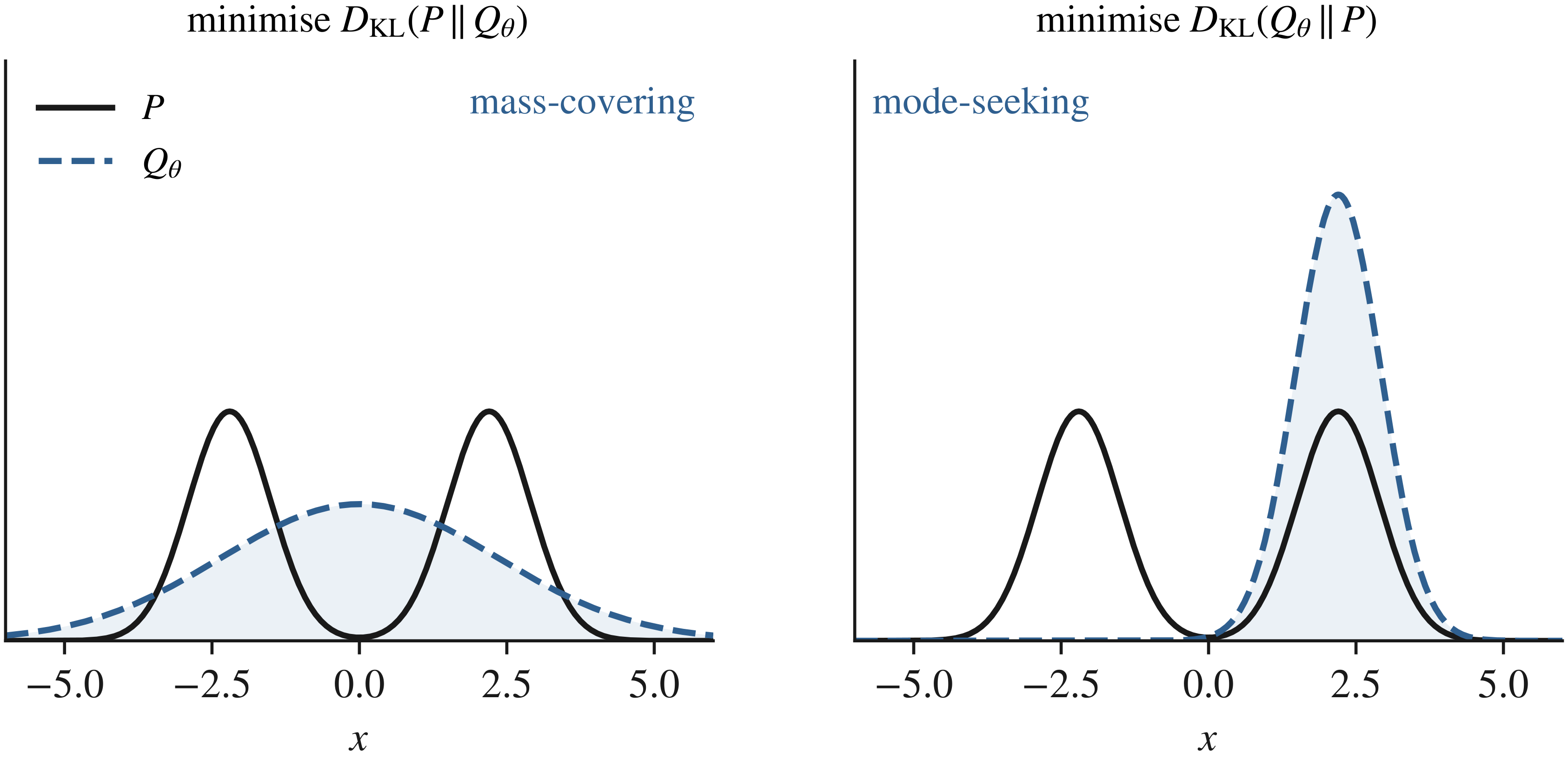
the reverse Kullback–Leibler divergence, finite only when Q \ll P. The asymmetry is not a technicality: minimising D_{\mathrm{KL}}(P \Vert Q_\theta) over \theta penalises putting no mass where P has some, so the fitted model spreads out to cover every mode; minimising D_{\mathrm{KL}}(Q_{\theta} \Vert P) penalises putting mass where P has none, so the fitted model contracts onto one mode and ignores the rest. Figure 1.4 shows the two fits side by side.
1.6.2 Total variation
The generator f(u) = \tfrac{1}{2}\lvert u - 1 \rvert is convex and vanishes at u = 1, so it defines an f-divergence. It is the one member of the family that is also a metric, and the one that will reappear in Section 1.8 from the other direction entirely.
Proposition 1.2 (Total variation) With f(u) = \tfrac{1}{2}\lvert u-1 \rvert,
D_{f}(P \Vert Q) = \tfrac{1}{2} \int \lvert p(x) - q(x) \rvert \, d\xi(x) = \sup_{A} \, \lvert P(A) - Q(A) \rvert =: \delta(P,Q) , \tag{1.12}
the supremum being over measurable sets A.
Proof. The first equality is immediate from Equation 1.7:
\int \tfrac{1}{2} \left\lvert \frac{p}{q} - 1 \right\rvert q \, d\xi = \tfrac{1}{2} \int \lvert p - q \rvert \, d\xi .
For the second, write r = p - q and let A^{\ast} = \{ x : p(x) > q(x) \}. Since P and Q are probability measures, \int r \, d\xi = 0, so
\int_{A^{\ast}} r \, d\xi = - \int_{(A^{\ast})^{c}} r \, d\xi = \int_{(A^{\ast})^{c}} \lvert r \rvert \, d\xi .
The integrand \lvert r \rvert equals r on A^{\ast} and -r off it, so
\int \lvert r \rvert \, d\xi = \int_{A^{\ast}} r \, d\xi + \int_{(A^{\ast})^{c}} \lvert r \rvert \, d\xi = 2 \int_{A^{\ast}} r \, d\xi ,
giving P(A^{\ast}) - Q(A^{\ast}) = \tfrac{1}{2}\int \lvert r \rvert \, d\xi. That attains the supremum. For the upper bound, any measurable A satisfies
\lvert P(A) - Q(A) \rvert = \left\lvert \int_{A} r \, d\xi \right\rvert \leq \max\left\{ \int_{A} r^{+} d\xi , \int_{A} r^{-} d\xi \right\} \leq \int r^{+} d\xi = \tfrac{1}{2} \int \lvert r \rvert \, d\xi ,
where the last equality uses \int r^{+} d\xi = \int r^{-} d\xi, itself a restatement of \int r \, d\xi = 0.
Unlike the Kullback–Leibler divergence, Equation 1.12 never exceeds 1 and never needs absolute continuity: the generator \tfrac{1}{2}\lvert u-1 \rvert grows linearly, so f(u)/u stays bounded. Boundedness will turn out to be exactly the problem rather than the cure.
1.6.3 Jensen–Shannon divergence
The Jensen–Shannon divergence symmetrises the Kullback–Leibler divergence by comparing both arguments against their average.
Definition 1.7 (Jensen–Shannon divergence) For probability measures P and Q, set M = \tfrac{1}{2}(P + Q). Then
D_{\mathrm{JS}}(P \Vert Q) := \tfrac{1}{2} D_{\mathrm{KL}}(P \Vert M) + \tfrac{1}{2} D_{\mathrm{KL}}(Q \Vert M) . \tag{1.13}
Symmetry is immediate, since M is unchanged by swapping P and Q. The substantive point is that Equation 1.13 is always finite, which the Kullback–Leibler divergence is not.
Lemma 1.2 (The mixture dominates both arguments) P \ll M and Q \ll M, so both Radon–Nikodym derivatives dP/dM and dQ/dM exist and Equation 1.13 is well defined for every pair P, Q.
Proof. Let A be measurable with M(A) = 0. By definition of M,
0 = M(A) = \tfrac{1}{2} P(A) + \tfrac{1}{2} Q(A) .
Both P(A) \geq 0 and Q(A) \geq 0, and a sum of non-negative terms vanishes only if each vanishes, so P(A) = Q(A) = 0. By Definition 1.1 this is exactly P \ll M and Q \ll M.
This is the whole advantage over the Kullback–Leibler divergence. To use D_{\mathrm{KL}}(P \Vert Q) we must know in advance that P \ll Q, which for a model distribution and an unknown data distribution we never do.
Proposition 1.3 (Jensen–Shannon is bounded) 0 \leq D_{\mathrm{JS}}(P \Vert Q) \leq \log 2, with the upper bound attained exactly when P and Q are mutually singular.
Proof. The lower bound is Proposition 1.1. For the upper bound, note that pointwise M = \tfrac{1}{2}(P+Q) \geq \tfrac{1}{2}P as measures, so dP/dM \leq 2 M-almost everywhere. Hence
D_{\mathrm{KL}}(P \Vert M) = \int \log\!\left( \frac{dP}{dM} \right) dP \leq \int \log 2 \, dP = \log 2 ,
and the same bound holds for D_{\mathrm{KL}}(Q \Vert M). Substituting both into Equation 1.13 gives D_{\mathrm{JS}} \leq \tfrac{1}{2}\log 2 + \tfrac{1}{2}\log 2 = \log 2.
Equality requires dP/dM = 2 P-almost everywhere. Because P + Q = 2M, the two derivatives satisfy dP/dM + dQ/dM = 2 M-almost everywhere, so on the set S = \{ dP/dM = 2 \} we have dQ/dM = 0 and therefore
Q(S) = \int_{S} \frac{dQ}{dM} \, dM = 0 ,
while P(S) = 1. So P and Q are carried by the disjoint sets S and S^{c}, which is mutual singularity. Conversely, if P and Q live on disjoint sets S and S^{c}, then on S we have M = \tfrac{1}{2}P and dP/dM = 2, and symmetrically on S^{c}, so both divergences equal \log 2.
Finally we connect Equation 1.13 back to Definition 1.6, and here the lecture’s two slides do not quite agree with each other.
Proposition 1.4 (The Jensen–Shannon generator carries a factor of two) Let f_{\mathrm{JS}}(u) = (u+1)\log\frac{2}{u+1} + u \log u. Then f_{\mathrm{JS}} is convex with f_{\mathrm{JS}}(1) = 0, and
D_{f_{\mathrm{JS}}}(P \Vert Q) = 2 \, D_{\mathrm{JS}}(P \Vert Q) . \tag{1.14}
Proof. That f_{\mathrm{JS}}(1) = 2\log 1 + 1 \cdot \log 1 = 0 is direct. For convexity, differentiate twice on u > 0:
f_{\mathrm{JS}}'(u) = \log \frac{2}{u+1} - 1 + \log u + 1 = \log \frac{2u}{u+1} , \qquad f_{\mathrm{JS}}''(u) = \frac{1}{u} - \frac{1}{u+1} = \frac{1}{u(u+1)} > 0 .
For the identity, substitute into Equation 1.8 with u = P(x)/Q(x) and clear denominators:
\begin{aligned} D_{f_{\mathrm{JS}}}(P \Vert Q) &= \sum_{x} Q \left[ \left( \frac{P}{Q} + 1 \right) \log \frac{2}{\frac{P}{Q} + 1} + \frac{P}{Q} \log \frac{P}{Q} \right] \\ &= \sum_{x} \left[ (P + Q) \log \frac{2Q}{P + Q} + P \log \frac{P}{Q} \right] . \end{aligned}
Now M = \tfrac{1}{2}(P+Q) gives \dfrac{2Q}{P+Q} = \dfrac{Q}{M}, so
\begin{aligned} D_{f_{\mathrm{JS}}}(P \Vert Q) &= \sum_{x} \left[ P \log \frac{Q}{M} + Q \log \frac{Q}{M} + P \log \frac{P}{Q} \right] \\ &= \sum_{x} \left[ P \log \!\left( \frac{Q}{M} \cdot \frac{P}{Q} \right) + Q \log \frac{Q}{M} \right] \\ &= \sum_{x} P \log \frac{P}{M} + \sum_{x} Q \log \frac{Q}{M} \\ &= D_{\mathrm{KL}}(P \Vert M) + D_{\mathrm{KL}}(Q \Vert M) , \end{aligned}
which by Equation 1.13 is 2 D_{\mathrm{JS}}(P \Vert Q).
The factor of two is not an error in either statement; it is a collision of two conventions. Equation 1.13 is the information-theoretic normalisation, under which the divergence is bounded by \log 2 and equals the mutual information between a sample and a fair coin choosing which of P and Q produced it. f_{\mathrm{JS}} is the generator tabulated in the f-GAN literature, which omits the \tfrac{1}{2} so that the associated variational objective matches the original GAN loss up to an additive \log 4. This chapter uses Equation 1.13 throughout, so that the bound of Proposition 1.3 reads \log 2; a reader comparing against a table of f-divergence generators should expect the other normalisation and divide by two.
1.7 Disjoint supports and the vanishing gradient
Everything so far has quietly assumed that the density ratio p/q means something. This section shows what happens when it does not, which for generative models is the typical case rather than a pathology. The conclusion is that every f-divergence saturates at a constant that does not depend on how far apart the two distributions are, and that a constant has no gradient.
To say this cleanly we need the standard extension of Definition 1.6 to pairs that are not absolutely continuous. Let P = P^{\mathrm{ac}} + P^{\perp} be the Lebesgue decomposition of P with respect to Q, and define the recession slope
f'(\infty) := \lim_{u \to \infty} \frac{f(u)}{u} \in (-\infty, +\infty] , \tag{1.15}
which exists in the extended reals because f is convex. The f-divergence is then
D_{f}(P \Vert Q) := \int f\!\left( \frac{dP^{\mathrm{ac}}}{dQ} \right) dQ \; + \; f'(\infty) \, P^{\perp}(\Omega) , \tag{1.16}
which agrees with Equation 1.6 when P \ll Q, since then P^{\perp} = 0.
Theorem 1.2 (Saturation on disjoint supports) Let P and Q be mutually singular probability measures, written P \perp Q. Then for every generator f,
D_{f}(P \Vert Q) = f(0) + f'(\infty) , \tag{1.17}
a constant depending only on f and not on P or Q.
Proof. Mutual singularity means there is a measurable set S with P(S) = 1 and Q(S) = 0. Then P is carried by S and Q by S^{c}, so the Lebesgue decomposition of P with respect to Q is P^{\mathrm{ac}} = 0 and P^{\perp} = P, whence dP^{\mathrm{ac}}/dQ = 0 Q-almost everywhere. Substituting into Equation 1.16,
D_{f}(P \Vert Q) = \int f(0) \, dQ + f'(\infty) \, P(\Omega) = f(0) \cdot 1 + f'(\infty) \cdot 1 ,
since P and Q are probability measures.
Evaluating Equation 1.17 for the generators tabulated earlier gives the saturation values directly, and they agree with the bounds proved above.
| Divergence | f(0) | f'(\infty) | Value when P \perp Q |
|---|---|---|---|
| Kullback–Leibler | 0 | +\infty | +\infty |
| Reverse Kullback–Leibler | +\infty | 0 | +\infty |
| Pearson \chi^{2} | 1 | +\infty | +\infty |
| Squared Hellinger | 1 | 1 | 2 |
| Total variation | \tfrac{1}{2} | \tfrac{1}{2} | 1 |
| Jensen–Shannon (as f_{\mathrm{JS}}) | \log 2 | \log 2 | 2 \log 2 |
The last row is a useful consistency check on Proposition 1.4: dividing the saturation value 2 \log 2 by the factor of two recovers exactly the bound \log 2 of Proposition 1.3, attained precisely on mutually singular pairs. The Pearson \chi^{2} row is the one generator the chapter tabulates but never works through; Section 1.15.1 does so.
1.7.1 What this costs a generator
Example 1.1 (Two parallel segments) Let Z \sim \mathrm{Uniform}[0,1] and work in \mathbb{R}^{2}. Define \mu_{0} to be the law of (0, Z) and, for \theta \in \mathbb{R}, define \mu_{\theta} to be the law of (\theta, Z). Each is uniform on a vertical unit segment, and for \theta \neq 0 the two segments are disjoint. Then
W_{1}(\mu_{0}, \mu_{\theta}) = \lvert \theta \rvert , \qquad D_{\mathrm{JS}}(\mu_{0} \Vert \mu_{\theta}) = \begin{cases} \log 2 , & \theta \neq 0 \\ 0 , & \theta = 0 \end{cases} ,
\delta(\mu_{0}, \mu_{\theta}) = \begin{cases} 1 , & \theta \neq 0 \\ 0 , & \theta = 0 \end{cases} , \qquad D_{\mathrm{KL}}(\mu_{0} \Vert \mu_{\theta}) = \begin{cases} +\infty , & \theta \neq 0 \\ 0 , & \theta = 0 . \end{cases}
Proof. For \theta \neq 0 the supports are the disjoint segments \{0\} \times [0,1] and \{\theta\} \times [0,1], so \mu_{0} \perp \mu_{\theta} and the last three claims are Theorem 1.2 read off the table, with the Jensen–Shannon entry divided by two to match the normalisation of Equation 1.13. At \theta = 0 the two measures coincide and every divergence vanishes by Proposition 1.1.
For W_{1}, whose definition is Definition 1.10 below, take the coupling \pi induced by the map (0,z) \mapsto (\theta, z), that is, the law of \bigl( (0,Z), (\theta,Z) \bigr). Its marginals are \mu_{0} and \mu_{\theta} by construction, and its cost is
\mathbb{E} \left\lVert (0,Z) - (\theta,Z) \right\rVert = \mathbb{E} \lvert \theta \rvert = \lvert \theta \rvert ,
so W_{1}(\mu_{0}, \mu_{\theta}) \leq \lvert \theta \rvert. Conversely, let \pi be any coupling and let (X, Y) \sim \pi. Writing X_{1}, Y_{1} for first coordinates, X_{1} = 0 almost surely and Y_{1} = \theta almost surely, so \lVert X - Y \rVert \geq \lvert X_{1} - Y_{1} \rvert = \lvert \theta \rvert pointwise, and taking expectations gives \mathbb{E}\lVert X - Y \rVert \geq \lvert \theta \rvert. Hence W_{1}(\mu_{0}, \mu_{\theta}) \geq \lvert \theta \rvert, and the two bounds agree.
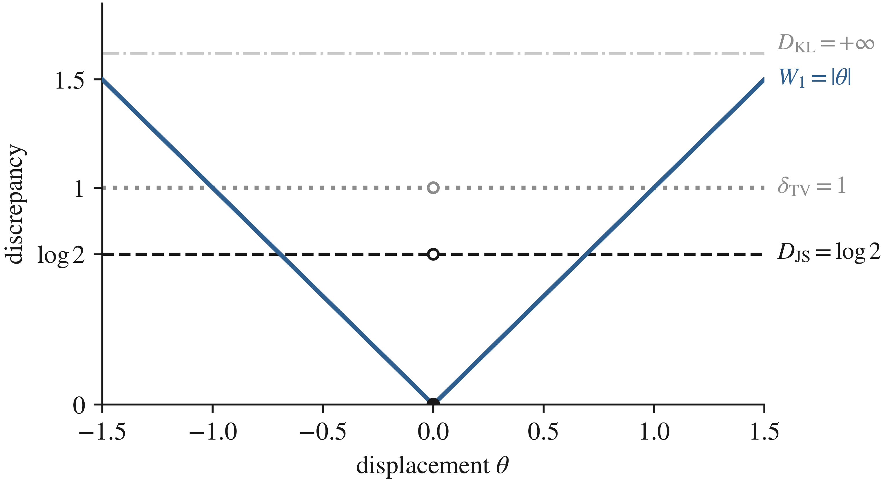
Figure 1.5 is the picture to keep. Suppose we train a generator whose only parameter is the horizontal offset \theta, and we descend the divergence in \theta. Under W_{1} the objective is \lvert \theta \rvert, with derivative \mathrm{sign}(\theta): from any starting point the gradient points at the answer. Under the Jensen–Shannon divergence the objective is the constant \log 2 for every \theta \neq 0, so its derivative is zero everywhere except at the single point we are trying to find. The optimiser receives no information at all. Under the Kullback–Leibler divergence the objective is not even finite.
This is not an artefact of a one-dimensional toy. By Equation 1.1 the model distribution \mu_{\theta} is supported on G_{\theta}(\mathcal{Y}), the image of a latent space of dimension perhaps 100, embedded in a pixel space of dimension perhaps 10^{5}; and the data are taken to lie on a manifold of comparably small dimension. Two sets of dimension 100 inside \mathbb{R}^{10^{5}} that are not deliberately arranged to meet will be mutually singular, so Theorem 1.2 applies at essentially every \theta, not just at isolated ones. A generator trained against an f-divergence is therefore relying on the discriminator never becoming very good — an unstable thing to rely on, and the observed behaviour of the original GAN.
Two escapes exist. One is to stop comparing densities pointwise and start comparing expectations of test functions, which is Section 1.8. The other is to measure how far mass must physically move, which is Section 1.10 onwards. They turn out to be the same escape, and they meet in Theorem 1.7.
1.8 Integral probability metrics
An f-divergence asks how the two distributions differ at each point. An integral probability metric asks instead how differently they answer a restricted set of questions.
Definition 1.8 (Integral probability metric) Let \mathcal{F} be a class of real measurable functions on \mathcal{X}. The integral probability metric associated with \mathcal{F} is
d_{\mathcal{F}}(\mu, \nu) := \sup_{h \in \mathcal{F}} \left\lvert \int_{\mathcal{X}} h \, d\mu - \int_{\mathcal{X}} h \, d\nu \right\rvert . \tag{1.18}
The name “dual-norm view” comes from reading Equation 1.18 as a norm on the signed measure \mu - \nu. Probability measures pair with bounded functions by integration, so \mu - \nu acts as a linear functional on the space of test functions; Equation 1.18 is the operator norm of that functional, measured over the unit ball \mathcal{F}. Different choices of \mathcal{F} are different norms on the same object, and, as we are about to see, three familiar quantities are three choices. How literally that dual-norm reading may be taken, and which topology each choice induces, are examined in Section 1.15.2.
Throughout we take \mathcal{F} symmetric, \mathcal{F} = -\mathcal{F}, as all three classes below are; the absolute value in Equation 1.18 may then be dropped, since h and -h both compete in the supremum.
Proposition 1.5 (Integral probability metrics are pseudo-metrics) Let every h \in \mathcal{F} be integrable with respect to both measures. Then d_{\mathcal{F}} is non-negative, symmetric, vanishes when \mu = \nu, and satisfies the triangle inequality. It is a metric on \mathcal{P}(\mathcal{X}) if and only if \mathcal{F} is measure-determining, meaning that \int h \, d\mu = \int h \, d\nu for all h \in \mathcal{F} implies \mu = \nu.
Proof. Non-negativity is clear, as is d_{\mathcal{F}}(\mu,\mu) = 0. Symmetry holds because the absolute value is unchanged when \mu and \nu are exchanged. For the triangle inequality, fix h \in \mathcal{F} and any third measure \rho; then
\left\lvert \int h \, d\mu - \int h \, d\nu \right\rvert \leq \left\lvert \int h \, d\mu - \int h \, d\rho \right\rvert + \left\lvert \int h \, d\rho - \int h \, d\nu \right\rvert \leq d_{\mathcal{F}}(\mu,\rho) + d_{\mathcal{F}}(\rho,\nu) .
The right-hand side does not depend on h, so taking the supremum over h \in \mathcal{F} on the left preserves the inequality.
Finally, d_{\mathcal{F}}(\mu,\nu) = 0 says exactly that \int h \, d\mu = \int h \, d\nu for every h \in \mathcal{F}. That this forces \mu = \nu is the definition of measure-determining, so the second axiom of Definition 1.3 holds precisely under that hypothesis.
Note how little was needed: no density ratio, no absolute continuity, and no common dominating measure. This is why integral probability metrics survive the situation that defeats Section 1.7.
1.8.1 Three instances
Total variation. Take \mathcal{F} to be the indicators \{ \mathbf{1}_{A} : A \text{ measurable} \}. Then \int \mathbf{1}_{A} d\mu - \int \mathbf{1}_{A} d\nu = \mu(A) - \nu(A), so Equation 1.18 reduces to \sup_{A} \lvert \mu(A) - \nu(A) \rvert, which is \delta(\mu,\nu) by Proposition 1.2. Taking instead the sup-norm ball \{ h : \lVert h \rVert_{\infty} \leq 1 \} gives 2\delta(\mu,\nu), since the supremum is attained at h = \mathrm{sign}(p - q).
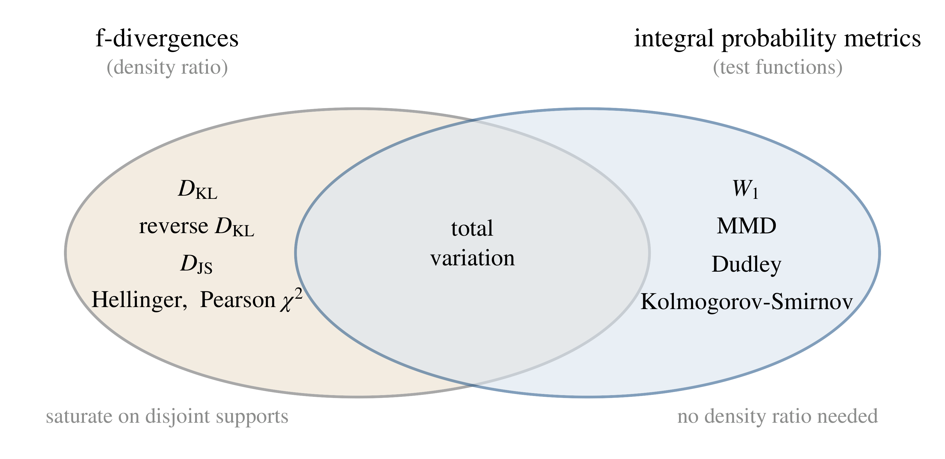
So total variation belongs to both families. That is not a coincidence about our proof, and it is essentially the only overlap: up to a constant multiple, total variation is the unique non-trivial statistical distance that is both an f-divergence and an integral probability metric, as Figure 1.6 records.
Wasserstein-1. Take \mathcal{F} = \mathrm{Lip}_{1}(\mathcal{X}) from Definition 1.5. The resulting integral probability metric is W_{1}. This is the Kantorovich–Rubinstein theorem and it is genuinely a theorem rather than a definition, because W_{1} is defined in Definition 1.10 as an infimum over couplings with no test functions in sight. We prove it as Theorem 1.7, once duality is available.
Maximum mean discrepancy. Let k be a positive-definite kernel on \mathcal{X} and \mathcal{H}_{k} its reproducing kernel Hilbert space, so that h(x) = \langle h, k(\cdot, x) \rangle_{\mathcal{H}_{k}} for every h \in \mathcal{H}_{k}. Take \mathcal{F} to be the unit ball \{ h : \lVert h \rVert_{\mathcal{H}_{k}} \leq 1 \}.
Proposition 1.6 (Maximum mean discrepancy) Assume \int \sqrt{k(x,x)} \, d\mu(x) and \int \sqrt{k(y,y)} \, d\nu(y) are finite, and define the mean embeddings m_{\mu} = \int k(\cdot, x) \, d\mu(x) and m_{\nu} = \int k(\cdot, y) \, d\nu(y) in \mathcal{H}_{k}. Then
\mathrm{MMD}(\mu,\nu) := d_{\mathcal{F}}(\mu,\nu) = \lVert m_{\mu} - m_{\nu} \rVert_{\mathcal{H}_{k}} , \tag{1.19}
and
\mathrm{MMD}^{2}(\mu,\nu) = \mathbb{E}_{x,x' \sim \mu} k(x,x') - 2 \, \mathbb{E}_{x \sim \mu, \, y \sim \nu} k(x,y) + \mathbb{E}_{y,y' \sim \nu} k(y,y') . \tag{1.20}
Proof. By the reproducing property and the finiteness assumption, integration against \mu is an inner product with the mean embedding:
\int h \, d\mu = \int \langle h, k(\cdot,x) \rangle_{\mathcal{H}_{k}} \, d\mu(x) = \left\langle h, \int k(\cdot,x) \, d\mu(x) \right\rangle_{\mathcal{H}_{k}} = \langle h, m_{\mu} \rangle_{\mathcal{H}_{k}} ,
the exchange of integral and inner product being justified by the same finiteness assumption. Subtracting the same identity for \nu,
\int h \, d\mu - \int h \, d\nu = \langle h, m_{\mu} - m_{\nu} \rangle_{\mathcal{H}_{k}} .
Taking the supremum of the absolute value over the unit ball is the definition of the dual norm in a Hilbert space, which by Cauchy–Schwarz equals \lVert m_{\mu} - m_{\nu} \rVert_{\mathcal{H}_{k}}, attained at h = (m_{\mu} - m_{\nu}) / \lVert m_{\mu} - m_{\nu} \rVert. That is Equation 1.19.
For Equation 1.20, expand the squared norm and use the reproducing property once more:
\langle m_{\mu}, m_{\nu} \rangle_{\mathcal{H}_{k}} = \left\langle \int k(\cdot,x) d\mu(x), \int k(\cdot,y) d\nu(y) \right\rangle = \int \!\! \int \langle k(\cdot,x), k(\cdot,y) \rangle \, d\mu \, d\nu = \int \!\! \int k(x,y) \, d\mu \, d\nu ,
and similarly for \langle m_{\mu}, m_{\mu} \rangle and \langle m_{\nu}, m_{\nu} \rangle. Substituting into \lVert m_{\mu} - m_{\nu} \rVert^{2} = \langle m_{\mu},m_{\mu}\rangle - 2\langle m_{\mu},m_{\nu}\rangle + \langle m_{\nu},m_{\nu}\rangle gives the result.
Equation 1.20 is what makes the maximum mean discrepancy practical: it is written entirely in terms of expectations of the kernel, so it can be estimated from two samples without any density estimate and without solving the supremum. The two standard estimators, and the condition on the kernel under which the maximum mean discrepancy separates distributions at all, are in Section 1.15.3.
This is the discrepancy behind the moment-matching generative models, and it is where McGAN and MMD-GAN enter in the next lecture.
1.9 Wasserstein distances
We now build the second family. Instead of comparing \mu and \nu where they sit, we ask what it would cost to carry the mass of one onto the other. The bookkeeping device for “carrying mass” is a joint distribution.
Definition 1.9 (Coupling) Let \mu \in \mathcal{P}(\mathcal{X}) and \nu \in \mathcal{P}(\mathcal{Y}). A coupling of \mu and \nu is a probability measure \pi on \mathcal{X} \times \mathcal{Y} whose marginals are \mu and \nu:
\pi(A \times \mathcal{Y}) = \mu(A) , \qquad \pi(\mathcal{X} \times B) = \nu(B) \tag{1.21}
for all measurable A \subseteq \mathcal{X}, B \subseteq \mathcal{Y}. The set of couplings is written \Pi(\mu,\nu).
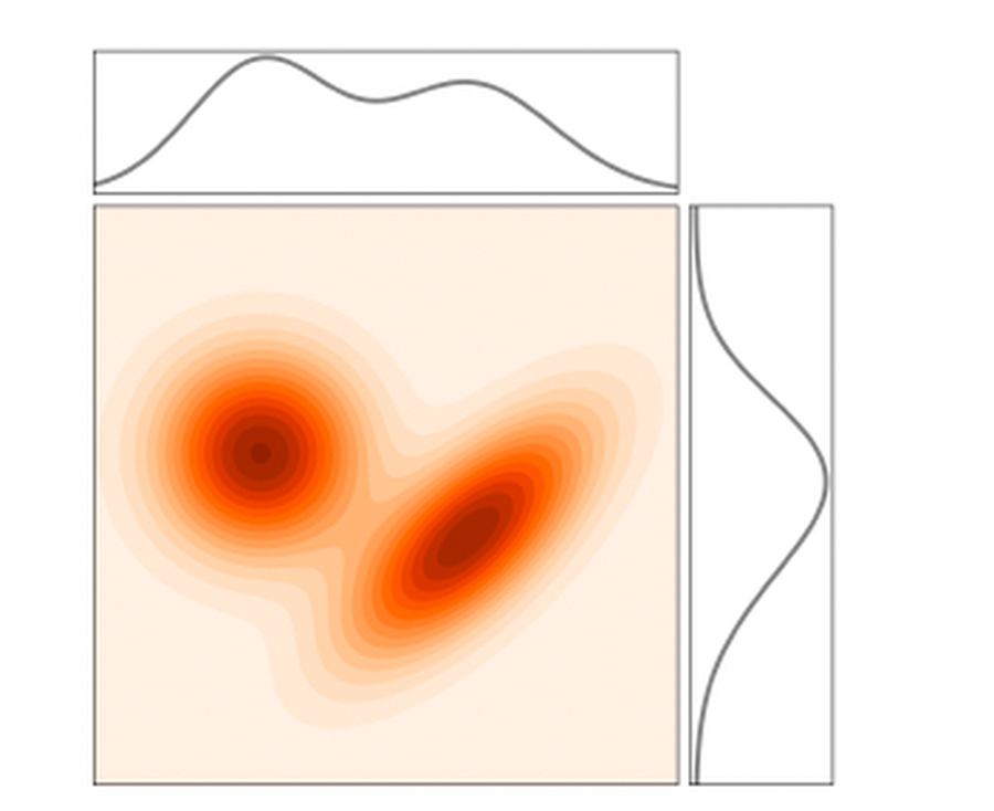
Read \pi(dx,dy) as the amount of mass moved from x to y. The two constraints in Equation 1.21 say that everything sent out of x adds up to what \mu had there, and everything arriving at y adds up to what \nu needs there. The set \Pi(\mu,\nu) is never empty: the product measure \mu \otimes \nu, which ignores where mass came from, is always a coupling.
Definition 1.10 (Wasserstein distance) Let (\mathcal{M}, d) be a Polish metric space and let p \geq 1. For \mu, \nu \in \mathcal{P}(\mathcal{M}) with finite p-th moments, the p-th Wasserstein distance is
W_{p}(\mu,\nu) := \left( \inf_{\pi \in \Pi(\mu,\nu)} \int_{\mathcal{M} \times \mathcal{M}} d(x,y)^{p} \, d\pi(x,y) \right)^{1/p} = \left( \inf_{\pi \in \Pi(\mu,\nu)} \mathbb{E}_{\pi} \bigl[ d(X,Y)^{p} \bigr] \right)^{1/p} . \tag{1.22}
For p = 1 this is the earth-mover distance: the least total amount of “mass times distance” needed to rearrange one pile of earth into the other. The name is worth taking literally, because it is the source of the intuition that Figure 1.5 makes precise — moving two separated piles closer together reduces the cost continuously, whereas asking whether they overlap gives the same answer until the instant they touch.
That Equation 1.22 really is a metric, and not merely a divergence, is the structural fact that distinguishes this family from Section 1.6.
Theorem 1.3 (Wasserstein is a metric) For p \geq 1, W_{p} satisfies all four axioms of Definition 1.3 on the set of probability measures on \mathcal{M} with finite p-th moments.
Proof. Non-negativity is immediate, since d^{p} \geq 0.
Symmetry. If \pi \in \Pi(\mu,\nu), let S(x,y) = (y,x) and put \pi' = S_{\#}\pi. By Equation 1.4 its marginals are those of \pi in the opposite order, so \pi' \in \Pi(\nu,\mu), and by Lemma 1.1 its cost is \int d(y,x)^{p} d\pi = \int d(x,y)^{p} d\pi because d is symmetric. So S_{\#} is a cost-preserving bijection between \Pi(\mu,\nu) and \Pi(\nu,\mu), and the two infima agree.
Identity of indiscernibles. If \mu = \nu, the coupling \pi = (\mathrm{id},\mathrm{id})_{\#}\mu concentrated on the diagonal has cost \int d(x,x)^{p} d\mu = 0, so W_{p}(\mu,\mu) = 0. Conversely suppose W_{p}(\mu,\nu) = 0 and let \pi be an optimal coupling, which exists by Theorem 1.5 — this is the one place the proof uses the standing assumption of Definition 1.10 that \mathcal{M} is Polish, the cost d^{p} being continuous and hence lower semicontinuous. Then \int d(x,y)^{p} d\pi = 0 with a non-negative integrand, so d(x,y) = 0 and hence x = y for \pi-almost every pair; that is, \pi is concentrated on the diagonal \Delta = \{(x,x)\}, a measurable set since \mathcal{M} is metric. As \pi(\Delta) = 1, intersecting with \Delta leaves any \pi-measure unchanged, and for measurable A the sets (A \times \mathcal{M}) \cap \Delta and (\mathcal{M} \times A) \cap \Delta coincide — both are \{(x,x) : x \in A\}. Hence
\mu(A) = \pi(A \times \mathcal{M}) = \pi(\mathcal{M} \times A) = \nu(A) ,
and \mu = \nu.
Triangle inequality. Let \mu_{1}, \mu_{2}, \mu_{3} be given and take \pi_{12} \in \Pi(\mu_{1},\mu_{2}) and \pi_{23} \in \Pi(\mu_{2},\mu_{3}). The gluing lemma provides a measure \sigma on \mathcal{M} \times \mathcal{M} \times \mathcal{M} whose projection onto the first two coordinates is \pi_{12} and onto the last two is \pi_{23}; it is built by disintegrating both couplings over their shared marginal \mu_{2} and setting d\sigma(x_{1},x_{2},x_{3}) = d\pi_{12}(x_{1} \mid x_{2}) \, d\pi_{23}(x_{3} \mid x_{2}) \, d\mu_{2}(x_{2}). Its projection onto the first and third coordinates is some \pi_{13} \in \Pi(\mu_{1},\mu_{3}). Then
\begin{aligned} W_{p}(\mu_{1},\mu_{3}) &\leq \left( \int d(x_{1},x_{3})^{p} \, d\sigma \right)^{1/p} \\ &\leq \left( \int \bigl( d(x_{1},x_{2}) + d(x_{2},x_{3}) \bigr)^{p} d\sigma \right)^{1/p} \\ &\leq \left( \int d(x_{1},x_{2})^{p} d\sigma \right)^{1/p} + \left( \int d(x_{2},x_{3})^{p} d\sigma \right)^{1/p} \\ &= \left( \int d^{p} \, d\pi_{12} \right)^{1/p} + \left( \int d^{p} \, d\pi_{23} \right)^{1/p} , \end{aligned}
using the triangle inequality for d in the second step and Minkowski’s inequality in L^{p}(\sigma) in the third. Taking the infimum over \pi_{12} and \pi_{23} separately gives W_{p}(\mu_{1},\mu_{3}) \leq W_{p}(\mu_{1},\mu_{2}) + W_{p}(\mu_{2},\mu_{3}).
By Jensen’s inequality W_{1} \leq W_{p} for p \geq 1, so the Wasserstein distances form an increasing family. We will use W_{1} almost exclusively, because it is the one with a dual formulation simple enough to implement. Being a metric is not by itself what matters for Section 1.14 — which topology the metric induces is — and Section 1.15.4 settles that.
1.10 Monge’s formulation
Historically the transport problem was posed not with couplings but with maps: each grain of earth is assigned one destination.
Definition 1.11 (Transportation map) A measurable T : \mathcal{X} \to \mathcal{Y} transports \mu \in \mathcal{P}(\mathcal{X}) to \nu \in \mathcal{P}(\mathcal{Y}) if
\nu(B) = \mu\bigl( T^{-1}(B) \bigr) \quad \text{for all measurable } B , \tag{1.23}
that is, if \nu = T_{\#}\mu in the sense of Definition 1.2.
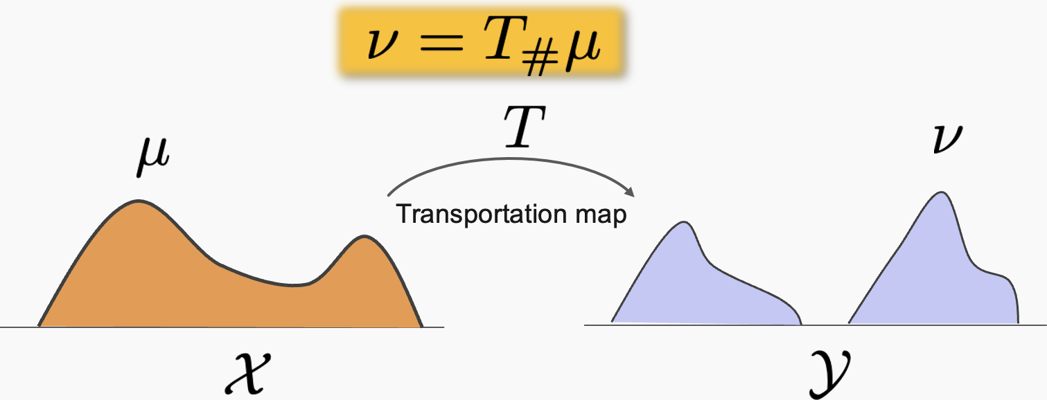
Figure 1.8 also shows what will go wrong. A map sends each source point somewhere; it cannot send one point to two places. When \nu has mass where no single destination will do — the two humps on the right, fed from one hump on the left — a transport map may fail to exist at all, which is Proposition 1.7 below.
Definition 1.12 (Monge’s problem) Given a cost c : \mathcal{X} \times \mathcal{Y} \to [0,\infty], Monge’s optimal transport problem is
\min_{T} \; \mathbb{M}(T) := \int_{\mathcal{X}} c\bigl( x, T(x) \bigr) \, d\mu(x) \qquad \text{subject to} \quad \nu = T_{\#}\mu . \tag{1.24}
The objective is benign; the constraint is not. The map T \mapsto T_{\#}\mu is nonlinear, and the feasible set \{ T : T_{\#}\mu = \nu \} is not convex: if T_{0} and T_{1} both push \mu to \nu, there is no reason for \tfrac{1}{2}(T_{0}+T_{1}) to do so. So Equation 1.24 cannot be attacked by the standard machinery of convex optimisation. Worse, it can be infeasible.
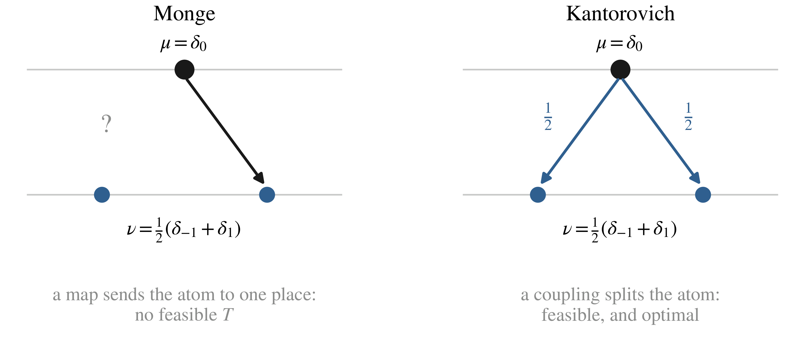
Proposition 1.7 (Monge’s problem may admit no solution) Let \mu = \delta_{0} on \mathbb{R} and \nu = \tfrac{1}{2}(\delta_{-1} + \delta_{1}). Then no measurable T satisfies T_{\#}\mu = \nu, so Equation 1.24 has no feasible point at all.
Proof. Suppose T_{\#}\mu = \nu. For any measurable B, Equation 1.23 gives \nu(B) = \mu(T^{-1}(B)) = \delta_{0}(T^{-1}(B)), which is 1 if 0 \in T^{-1}(B) and 0 otherwise. So \nu(B) \in \{0,1\} for every B. But \nu(\{1\}) = \tfrac{1}{2}, a contradiction.
The obstruction is plain once seen: a map sends the single atom at 0 somewhere, and it can only send it to one place, whereas \nu requires the mass to end up in two. A map cannot split mass. This is exactly what Section 1.11 repairs. Atoms are the crudest obstruction but not the only one; Section 1.15.5 gives two more, one of which shows that a non-atomic \mu does not make Monge’s problem well behaved either.
When a solution does exist, the one-dimensional case can be written down.
Theorem 1.4 (Transport on the line) Let \mu, \nu be probability measures on \mathbb{R} with continuous, strictly increasing distribution functions F and G. Then T = G^{-1} \circ F satisfies T_{\#}\mu = \nu, and for c(x,y) = \lvert x - y \rvert^{p} with p \geq 1 it is optimal, giving
W_{p}(\mu,\nu) = \left( \int_{0}^{1} \bigl\lvert F^{-1}(z) - G^{-1}(z) \bigr\rvert^{p} dz \right)^{1/p} = \left( \int_{\mathbb{R}} \bigl\lvert x - G^{-1}(F(x)) \bigr\rvert^{p} dF(x) \right)^{1/p} . \tag{1.25}
Proof. We prove the push-forward claim and the formula; optimality of the monotone map for convex costs is classical and we cite it rather than reprove it.
Fix y \in \mathbb{R}. Since G is continuous and strictly increasing, and likewise F,
\begin{aligned} (T_{\#}\mu)\bigl( (-\infty, y] \bigr) &= \mu\bigl( \{ x : G^{-1}(F(x)) \leq y \} \bigr) \\ &= \mu\bigl( \{ x : F(x) \leq G(y) \} \bigr) \\ &= \mu\bigl( \{ x : x \leq F^{-1}(G(y)) \} \bigr) \\ &= F\bigl( F^{-1}(G(y)) \bigr) = G(y) , \end{aligned}
where the second and third lines apply the increasing bijections G and F^{-1} to both sides of the inequality. So T_{\#}\mu and \nu have the same distribution function, hence are equal.
Given optimality, the cost of T is W_{p}^{p}. By Lemma 1.1 with the substitution x = F^{-1}(z), which carries Lebesgue measure on [0,1] to \mu,
\int_{\mathbb{R}} \lvert x - T(x) \rvert^{p} \, d\mu(x) = \int_{0}^{1} \bigl\lvert F^{-1}(z) - G^{-1}(F(F^{-1}(z))) \bigr\rvert^{p} dz = \int_{0}^{1} \bigl\lvert F^{-1}(z) - G^{-1}(z) \bigr\rvert^{p} dz ,
which is Equation 1.25.
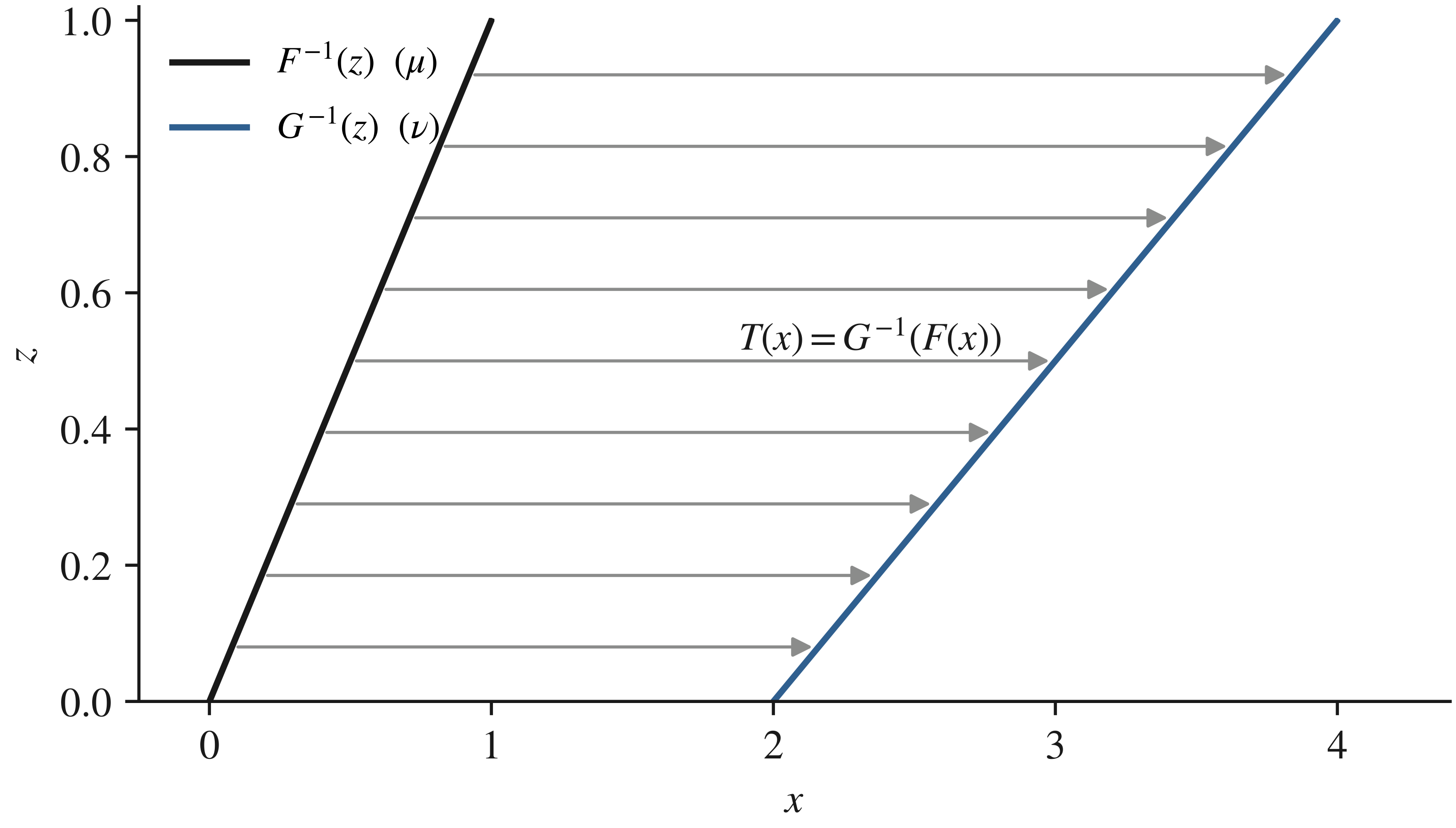
In Figure 1.9 the map is read off horizontally: fix a level z, find the point that \mu places at that quantile and the point that \nu places at the same quantile, and the arrow between them is where that parcel of mass goes. The next example carries this through with numbers.
Example 1.2 (A transport computed by hand) Let \mu = \mathrm{Uniform}[0,1] and \nu = \mathrm{Uniform}[2,4]. Then F(x) = x on [0,1] and G(y) = (y-2)/2 on [2,4], so F^{-1}(z) = z and G^{-1}(z) = 2 + 2z, and the optimal map is
T(x) = G^{-1}(F(x)) = 2 + 2x .
The map stretches the unit interval to twice its length and shifts it. By Equation 1.25 the transport costs are
W_{1} = \int_{0}^{1} \lvert z - (2+2z) \rvert \, dz = \int_{0}^{1} (2 + z) \, dz = \frac{5}{2} ,
W_{2} = \left( \int_{0}^{1} (2+z)^{2} \, dz \right)^{1/2} = \left( \frac{(2+z)^{3}}{3} \Big\vert_{0}^{1} \right)^{1/2} = \left( \frac{27 - 8}{3} \right)^{1/2} = \sqrt{\frac{19}{3}} \approx 2.5166 .
Two sanity checks. The value W_{1} = 5/2 equals the distance between the two means, 3 - 1/2, as it must here because T(x) - x = 2 + x never changes sign, so no mass moves against the flow. And W_{1} \leq W_{2}, as Jensen’s inequality requires.
The computation is short enough to check numerically, which is worth doing once to see that the coupling really is optimal and not merely feasible:
import numpy as np
from scipy.stats import wasserstein_distance

rng = np.random.default_rng(0)
x = rng.uniform(0.0, 1.0, 2_000_000)      # mu  = Uniform[0, 1]
y = rng.uniform(2.0, 4.0, 2_000_000)      # nu  = Uniform[2, 4]

print(wasserstein_distance(x, y))         # ~2.5000   matches W_1 = 5/2
print(np.mean(np.abs(x - (2 + 2 * x))))   # ~2.5000   cost of T(x) = 2 + 2x
print(np.sqrt(np.mean((x - (2 + 2 * x)) ** 2)))   # ~2.5166  matches W_2
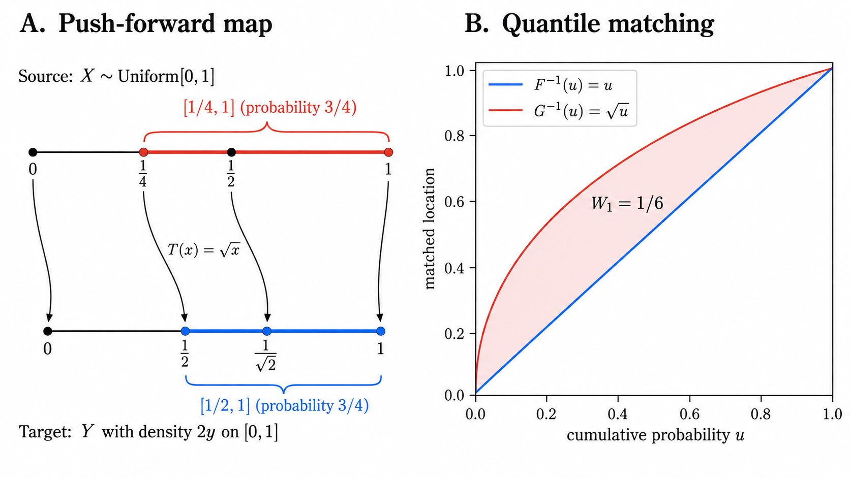
A second instance, with a map that is not affine, shows the two readings of Theorem 1.4 side by side.
1.11 Kantorovich’s relaxation
Kantorovich’s reformulation replaces the map by a coupling, and so allows mass at a single point to be split between several destinations. It is the problem we already wrote down as Equation 1.22, now stated for a general cost.
Definition 1.13 (Kantorovich’s problem) Given \mu \in \mathcal{P}(\mathcal{X}), \nu \in \mathcal{P}(\mathcal{Y}) and a cost c,
\mathbb{K}(\pi) := \int_{\mathcal{X} \times \mathcal{Y}} c(x,y) \, d\pi(x,y) , \qquad \min_{\pi \in \Pi(\mu,\nu)} \mathbb{K}(\pi) . \tag{1.26}
Three things improve at once. The objective is linear in \pi, the constraint set \Pi(\mu,\nu) is convex — a convex combination of couplings is a coupling, since Equation 1.21 is linear in \pi — and on finite spaces the whole thing is a linear program, the observation for which Kantorovich shared the 1975 Nobel Memorial Prize in Economics. Section 1.15.6 writes that program out, and reads off it both why the dual of Section 1.12 is the practical formulation and when the relaxation costs nothing.
Proposition 1.8 (The relaxation is genuine) Every transport map induces a coupling of the same cost, so
\min_{\pi \in \Pi(\mu,\nu)} \mathbb{K}(\pi) \; \leq \; \inf_{T : T_{\#}\mu = \nu} \mathbb{M}(T) . \tag{1.27}
Proof. Let T satisfy T_{\#}\mu = \nu and put \pi_{T} = (\mathrm{id}, T)_{\#} \mu, the law of (X, T(X)) for X \sim \mu. Its first marginal is \mu because the first coordinate of (\mathrm{id},T) is the identity, and its second marginal is T_{\#}\mu = \nu; so \pi_{T} \in \Pi(\mu,\nu). By Lemma 1.1 its cost is
\int c(x,y) \, d\pi_{T}(x,y) = \int c\bigl( x, T(x) \bigr) \, d\mu(x) = \mathbb{M}(T) .
Hence every value attained by \mathbb{M} is attained by \mathbb{K}, and the infimum over the larger set is no larger.
The inequality in Equation 1.27 can be strict, and Proposition 1.7 is the extreme case: the right-hand side is an infimum over the empty set, hence +\infty, while the left-hand side is finite. Indeed with \mu = \delta_{0}, \nu = \tfrac{1}{2}(\delta_{-1}+\delta_{1}) and c(x,y) = \lvert x-y \rvert, the only coupling is \pi = \tfrac{1}{2}\delta_{(0,-1)} + \tfrac{1}{2}\delta_{(0,1)} — it splits the atom, which no map can do — and its cost is 1. Figure 1.11 draws the two formulations on this example.
Unlike Monge’s problem, Kantorovich’s always has a solution.
Theorem 1.5 (Existence of an optimal coupling) Let \mathcal{X}, \mathcal{Y} be Polish spaces, \mu \in \mathcal{P}(\mathcal{X}), \nu \in \mathcal{P}(\mathcal{Y}), and let c : \mathcal{X} \times \mathcal{Y} \to [0,\infty] be lower semicontinuous. Then the minimum in Equation 1.26 is attained.
Proof. The set \Pi(\mu,\nu) is non-empty, since \mu \otimes \nu lies in it.
It is tight. Let \varepsilon > 0. By Ulam’s theorem, Borel probability measures on a Polish space are tight, so there are compact sets K_{1} \subseteq \mathcal{X} and K_{2} \subseteq \mathcal{Y} with \mu(K_{1}^{c}) \leq \varepsilon/2 and \nu(K_{2}^{c}) \leq \varepsilon/2. For any \pi \in \Pi(\mu,\nu), the complement of the compact set K_{1} \times K_{2} is contained in (K_{1}^{c} \times \mathcal{Y}) \cup (\mathcal{X} \times K_{2}^{c}), so by Equation 1.21
\pi\bigl( (K_{1} \times K_{2})^{c} \bigr) \leq \mu(K_{1}^{c}) + \nu(K_{2}^{c}) \leq \varepsilon .
The bound is uniform over \Pi(\mu,\nu), so the family is tight and, by Prokhorov’s theorem, relatively compact for the weak topology.
It is closed. If \pi_{n} \to \pi weakly with \pi_{n} \in \Pi(\mu,\nu), then for bounded continuous h on \mathcal{X}, the function (x,y) \mapsto h(x) is bounded and continuous on the product, so \int h(x) d\pi = \lim \int h(x) d\pi_{n} = \int h \, d\mu. Hence the first marginal of \pi is \mu, and symmetrically the second is \nu. So \Pi(\mu,\nu) is weakly closed, and with the previous paragraph, weakly compact.
The objective is lower semicontinuous. A non-negative lower semicontinuous c is the pointwise increasing limit of bounded continuous functions c_{k}. For each k, \pi \mapsto \int c_{k} \, d\pi is weakly continuous, and a supremum of continuous functions is lower semicontinuous, so \pi \mapsto \int c \, d\pi = \sup_{k} \int c_{k} \, d\pi is lower semicontinuous.
A lower semicontinuous function on a non-empty compact set attains its infimum, which is the claim.
1.12 Kantorovich duality
Equation 1.26 is a linear program over an infinite-dimensional convex set, so it has a dual. The dual turns out to be the formulation that generative models actually implement, because it needs only the two marginals and never the joint measure.
Theorem 1.6 (Kantorovich duality) Let \mu \in \mathcal{P}(\mathcal{X}), \nu \in \mathcal{P}(\mathcal{Y}) with \mathcal{X}, \mathcal{Y} Polish, and let c : \mathcal{X} \times \mathcal{Y} \to [0,+\infty] be lower semicontinuous. Define
\mathbb{J}(\varphi,\psi) = \int_{\mathcal{X}} \varphi \, d\mu + \int_{\mathcal{Y}} \psi \, d\nu , \qquad \Phi_{c} = \bigl\{ (\varphi,\psi) \in L^{1}(\mu) \times L^{1}(\nu) : \varphi(x) + \psi(y) \leq c(x,y) \bigr\} , \tag{1.28}
the inequality holding for \mu-almost every x and \nu-almost every y. Then
\min_{\pi \in \Pi(\mu,\nu)} \mathbb{K}(\pi) = \sup_{(\varphi,\psi) \in \Phi_{c}} \mathbb{J}(\varphi,\psi) . \tag{1.29}
Proof. Weak duality, in general. Let \pi \in \Pi(\mu,\nu) and (\varphi,\psi) \in \Phi_{c}. Because the marginals of \pi are \mu and \nu, integrating a function of x alone against \pi is the same as integrating it against \mu, and likewise for y and \nu. Hence
\mathbb{J}(\varphi,\psi) = \int \varphi(x) \, d\pi + \int \psi(y) \, d\pi = \int \bigl( \varphi(x) + \psi(y) \bigr) d\pi \leq \int c(x,y) \, d\pi = \mathbb{K}(\pi) ,
the inequality being the constraint defining \Phi_{c} integrated against the non-negative measure \pi. Taking the supremum on the left and the infimum on the right gives \sup \mathbb{J} \leq \min \mathbb{K}.
Strong duality, on finite spaces. Let \mathcal{X} = \{x_{1},\dots,x_{m}\} and \mathcal{Y} = \{y_{1},\dots,y_{n}\}, write \mu_{i}, \nu_{j}, c_{ij} and \pi_{ij}. The problem is the linear program
\min_{\pi \geq 0} \; \sum_{i,j} c_{ij}\pi_{ij} \quad \text{subject to} \quad \sum_{j} \pi_{ij} = \mu_{i} , \quad \sum_{i} \pi_{ij} = \nu_{j} .
Attach multipliers \varphi_{i} and \psi_{j} to the two families of constraints. The Lagrangian is
\begin{aligned} L(\pi,\varphi,\psi) &= \sum_{i,j} c_{ij}\pi_{ij} + \sum_{i} \varphi_{i}\Bigl( \mu_{i} - \sum_{j}\pi_{ij} \Bigr) + \sum_{j} \psi_{j}\Bigl( \nu_{j} - \sum_{i}\pi_{ij} \Bigr) \\ &= \sum_{i,j} \pi_{ij}\bigl( c_{ij} - \varphi_{i} - \psi_{j} \bigr) + \sum_{i} \varphi_{i}\mu_{i} + \sum_{j} \psi_{j}\nu_{j} . \end{aligned}
Minimising over \pi \geq 0 sends the first sum to -\infty unless every coefficient is non-negative, and gives 0 when they all are. So the dual function is finite exactly on \{ \varphi_{i} + \psi_{j} \leq c_{ij} \}, where it equals \mathbb{J}(\varphi,\psi), and the dual problem is \sup_{\Phi_{c}} \mathbb{J}. The primal is feasible, since \mu \otimes \nu is a coupling, and bounded below by 0, so linear programming duality gives equality of the two optimal values. The passage from finite spaces to Polish spaces is by approximation and is given in Villani, Theorem 1.3.
The dual constraint couples \varphi and \psi, but only in one direction: for a fixed \varphi there is a best possible \psi, and it can be written down.
Definition 1.14 (c-transform and c-concavity) For \varphi : \mathcal{X} \to \mathbb{R} and \psi : \mathcal{Y} \to \mathbb{R}, the c-transforms are
\varphi^{c}(y) := \inf_{x} \bigl\{ c(x,y) - \varphi(x) \bigr\} , \qquad \psi^{c}(x) := \inf_{y} \bigl\{ c(x,y) - \psi(y) \bigr\} . \tag{1.30}
A function \varphi is called c-concave if \varphi = \psi^{c} for some \psi. Optimal \varphi and \psi are called Kantorovich potentials.
Proposition 1.9 (The dual is a supremum over one potential) The dual problem in Equation 1.29 can be written
\sup_{(\varphi,\psi) \in \Phi_{c}} \mathbb{J}(\varphi,\psi) = \sup_{\varphi} \left\{ \int_{\mathcal{X}} \varphi \, d\mu + \int_{\mathcal{Y}} \varphi^{c} \, d\nu \right\} = \sup_{\psi} \left\{ \int_{\mathcal{X}} \psi^{c} \, d\mu + \int_{\mathcal{Y}} \psi \, d\nu \right\} , \tag{1.31}
and the supremum may be restricted to c-concave \varphi.
Proof. Fix \varphi. The constraint (\varphi,\psi) \in \Phi_{c} says \psi(y) \leq c(x,y) - \varphi(x) for every x, which is exactly \psi(y) \leq \varphi^{c}(y) by Equation 1.30. Since \mathbb{J} is increasing in \psi and \nu \geq 0, the largest admissible choice \psi = \varphi^{c} is optimal. This gives the first equality in Equation 1.31, and the second follows by the symmetric argument with the roles of the two potentials exchanged.
For the restriction, apply the transform twice. For every x and y, \varphi^{c}(y) \leq c(x,y) - \varphi(x), so c(x,y) - \varphi^{c}(y) \geq \varphi(x); taking the infimum over y gives
\varphi^{cc}(x) = \inf_{y} \bigl\{ c(x,y) - \varphi^{c}(y) \bigr\} \geq \varphi(x) .
So replacing \varphi by \varphi^{cc} never decreases \int \varphi \, d\mu. Applying the same inequality to \varphi^{c} gives \varphi^{ccc} \geq \varphi^{c}, while \varphi^{cc} \geq \varphi and the order-reversing nature of the transform give \varphi^{ccc} \leq \varphi^{c}; hence \varphi^{ccc} = \varphi^{c} and the second term is unchanged. So (\varphi^{cc}, \varphi^{c}) is admissible, has objective value at least that of (\varphi, \varphi^{c}), and \varphi^{cc} is c-concave by construction.
1.12.1 The Kantorovich–Rubinstein form of the Wasserstein-1 distance
Everything above holds for a general cost. For the particular cost c(x,y) = \lVert x - y \rVert the c-transform collapses, and the dual takes the form that W-GAN implements.
Lemma 1.3 (The c-transform of a 1-Lipschitz function) Let c(x,y) = \lVert x-y \rVert and let \varphi \in \mathrm{Lip}_{1}(\mathcal{X}). Then \varphi^{c} = -\varphi. Moreover a function is c-concave for this cost if and only if it is 1-Lipschitz, so the two classes coincide.
Proof. From Equation 1.30, choosing the particular point x = y in the infimum,
\varphi^{c}(y) = \inf_{x} \bigl\{ \lVert x-y \rVert - \varphi(x) \bigr\} \leq \lVert y-y \rVert - \varphi(y) = -\varphi(y) .
In the other direction, the 1-Lipschitz property gives \varphi(x) \leq \varphi(y) + \lVert x-y \rVert for every x, hence \lVert x-y \rVert - \varphi(x) \geq -\varphi(y) for every x, and taking the infimum over x,
\varphi^{c}(y) \geq -\varphi(y) .
The two inequalities give \varphi^{c} = -\varphi.
For the second claim, a c-concave function is by definition \psi^{c}(x) = \inf_{y}\{\lVert x-y \rVert - \psi(y)\}, an infimum of functions of x each of which is 1-Lipschitz; an infimum of a family of 1-Lipschitz functions is 1-Lipschitz wherever it is finite. Conversely a 1-Lipschitz \varphi is c-concave: taking \psi = -\varphi,
\psi^{c}(x) = \inf_{y} \bigl\{ \lVert x-y \rVert + \varphi(y) \bigr\} = \varphi(x) ,
because \varphi(y) \geq \varphi(x) - \lVert x-y \rVert makes every term at least \varphi(x), with equality at y = x. So the two classes coincide.
Theorem 1.7 (Kantorovich–Rubinstein) For c(x,y) = \lVert x-y \rVert,
W_{1}(\mu,\nu) = \min_{\pi \in \Pi(\mu,\nu)} \int \lVert x-y \rVert \, d\pi(x,y) = \sup_{\varphi \in \mathrm{Lip}_{1}(\mathcal{X})} \left\{ \int_{\mathcal{X}} \varphi \, d\mu - \int_{\mathcal{X}} \varphi \, d\nu \right\} . \tag{1.32}
Proof. The first equality is Definition 1.10 with p = 1 and d(x,y) = \lVert x-y \rVert. For the second, start from Equation 1.31, whose supremum may be taken over c-concave \varphi only. By Lemma 1.3 the c-concave functions for this cost are exactly the 1-Lipschitz ones, and on that class \varphi^{c} = -\varphi. Substituting,
\sup_{\varphi} \left\{ \int \varphi \, d\mu + \int \varphi^{c} \, d\nu \right\} = \sup_{\varphi \in \mathrm{Lip}_{1}} \left\{ \int \varphi \, d\mu - \int \varphi \, d\nu \right\} ,
and Theorem 1.6 equates this with the primal minimum.
Compare Equation 1.32 with Definition 1.8. The right-hand side is exactly the integral probability metric d_{\mathcal{F}} with \mathcal{F} = \mathrm{Lip}_{1}(\mathcal{X}) — the case promised in Section 1.8 and left unproved there. One step is needed to match the two expressions, since Definition 1.8 carries an absolute value and Equation 1.32 does not, and it is the symmetry assumed in Section 1.8: \mathrm{Lip}_{1} is closed under \varphi \mapsto -\varphi, so the supremum of the signed difference already equals the supremum of its absolute value.
The two families of statistical distance introduced in this chapter, one built from density ratios and one built from transport cost, meet at this single identity: W_{1} is simultaneously the cheapest way to move mass and the most a 1-Lipschitz test function can tell the two distributions apart.
The practical consequence is the one the lecture stresses. The primal in Equation 1.32 requires optimising over joint measures on \mathcal{X} \times \mathcal{X}, which is hopeless in high dimension. The dual requires only a single function \varphi and two expectations, each estimated from a sample of the corresponding marginal. Parameterise \varphi by a network constrained to be 1-Lipschitz, maximise the bracket in Equation 1.32, and the result estimates W_{1}; that network is the W-GAN critic, and the Lipschitz constraint is why it is clipped or gradient-penalised rather than left free.
1.13 Brenier’s theorem and the Gaussian case
Kantorovich’s relaxation buys existence at the price of abandoning maps. For the quadratic cost the map comes back, and with a great deal of extra structure.
Theorem 1.8 (Brenier) Let c(x,y) = \tfrac{1}{2}\lVert x-y \rVert^{2} on \mathbb{R}^{d}, and let \mu, \nu have finite second moments with \mu absolutely continuous with respect to Lebesgue measure. Then the optimal coupling of Equation 1.26 is unique and is induced by a map: there is a convex function u such that T = \nabla u satisfies T_{\#}\mu = \nu and \pi = (\mathrm{id}, T)_{\#}\mu is optimal. The map T is unique \mu-almost everywhere.
Proof. Expand the cost as c(x,y) = \tfrac{1}{2}\lVert x \rVert^{2} - \langle x,y \rangle + \tfrac{1}{2}\lVert y \rVert^{2} and change variables in the dual, setting
u(x) = \tfrac{1}{2}\lVert x \rVert^{2} - \varphi(x) , \qquad v(y) = \tfrac{1}{2}\lVert y \rVert^{2} - \psi(y) .
The dual constraint \varphi(x) + \psi(y) \leq c(x,y) becomes, after substituting and cancelling the two quadratic terms,
\langle x, y \rangle \leq u(x) + v(y) , \tag{1.33}
which is precisely the Fenchel–Young inequality for the pair u, v. In these variables the c-transform of Definition 1.14 is the Legendre transform, the relation \psi = \varphi^{c} reading v = u^{\ast}; this is worked out in Section 1.15.9. By Proposition 1.9 the supremum may be restricted to c-concave \varphi, which says here that u may be taken convex and lower semicontinuous with u = v^{\ast}.
Let \pi be an optimal coupling and (\varphi,\psi) optimal potentials, which exist for this cost because \tfrac{1}{2}\lVert x-y \rVert^{2} \leq \lVert x \rVert^{2} + \lVert y \rVert^{2} and both measures have finite second moments; Section 1.15.7 states the hypothesis in general. Weak duality was an integrated inequality, and equality of the two optimal values forces the non-negative integrand c - \varphi - \psi to vanish \pi-almost everywhere. So Equation 1.33 holds with equality for \pi-almost every (x,y):
\langle x,y \rangle = u(x) + v(y) .
The case of equality in the Fenchel–Young inequality is exactly y \in \partial u(x).
Next we check that u is finite and differentiable where the argument needs it. This deserves a step rather than an appeal: u = v^{\ast} is a supremum of affine functions and may perfectly well be +\infty off its effective domain. The equality above holds on a set of full \pi-measure, whose projection to the first coordinate therefore has full \mu-measure, and on it u(x) = \langle x,y \rangle - v(y) is finite. A convex function finite at each point of a set is finite on that set’s convex hull, so \mathrm{dom}\,u contains the convex hull K of a set of full \mu-measure. Since \mu \ll \mathrm{Lebesgue} cannot charge a hyperplane, K has non-empty interior; and the boundary of a convex set in \mathbb{R}^{d} is Lebesgue-null, so \mu(\partial K) = 0 and \mu-almost every x lies in \mathrm{int}\,K \subseteq \mathrm{int}\,\mathrm{dom}\,u. On the interior of its domain a finite convex function is locally Lipschitz, hence differentiable outside a set of Lebesgue measure zero by Rademacher’s theorem; that exceptional set is \mu-null too. So for \mu-almost every x the subdifferential is a single point, \partial u(x) = \{\nabla u(x)\}. Therefore y = \nabla u(x) for \pi-almost every (x,y), which says \pi is concentrated on the graph of T = \nabla u and hence \pi = (\mathrm{id},T)_{\#}\mu. Its second marginal is T_{\#}\mu and must equal \nu.
Uniqueness. Everything above applies to any optimal coupling, so each one is concentrated on the graph of the gradient of some convex potential. Let \pi and \pi' be optimal, carried by the graphs of T and T'. The objective Equation 1.26 is linear and \Pi(\mu,\nu) convex, so \tfrac{1}{2}(\pi + \pi') is optimal as well, hence also carried by a graph; a measure carried by a graph assigns to \mu-almost every x a single y, which forces T = T' \mu-almost everywhere. That gives uniqueness of both the map and the plan. Note what is not being claimed: the potential u itself is pinned down only up to an additive constant on each connected component of the interior of its domain, so on a disconnected support one may shift the components independently without changing anything. It is \nabla u, not u, that is unique.
The factor \tfrac{1}{2} in the cost is only a normalisation. Multiplying c by a positive constant rescales the optimal value but leaves the minimising coupling unchanged, so the map of Theorem 1.8 is equally optimal for c(x,y) = \lVert x-y \rVert^{2}, which is the cost Definition 1.10 uses at p = 2; the distance computed below is for that unhalved cost.
The theorem says something striking: the optimal transport map for the quadratic cost is never arbitrary. It is always the gradient of a convex potential, so it is a curl-free, monotone rearrangement of space. The lecture’s Gaussian formula is the simplest instance where the potential can be written in closed form.
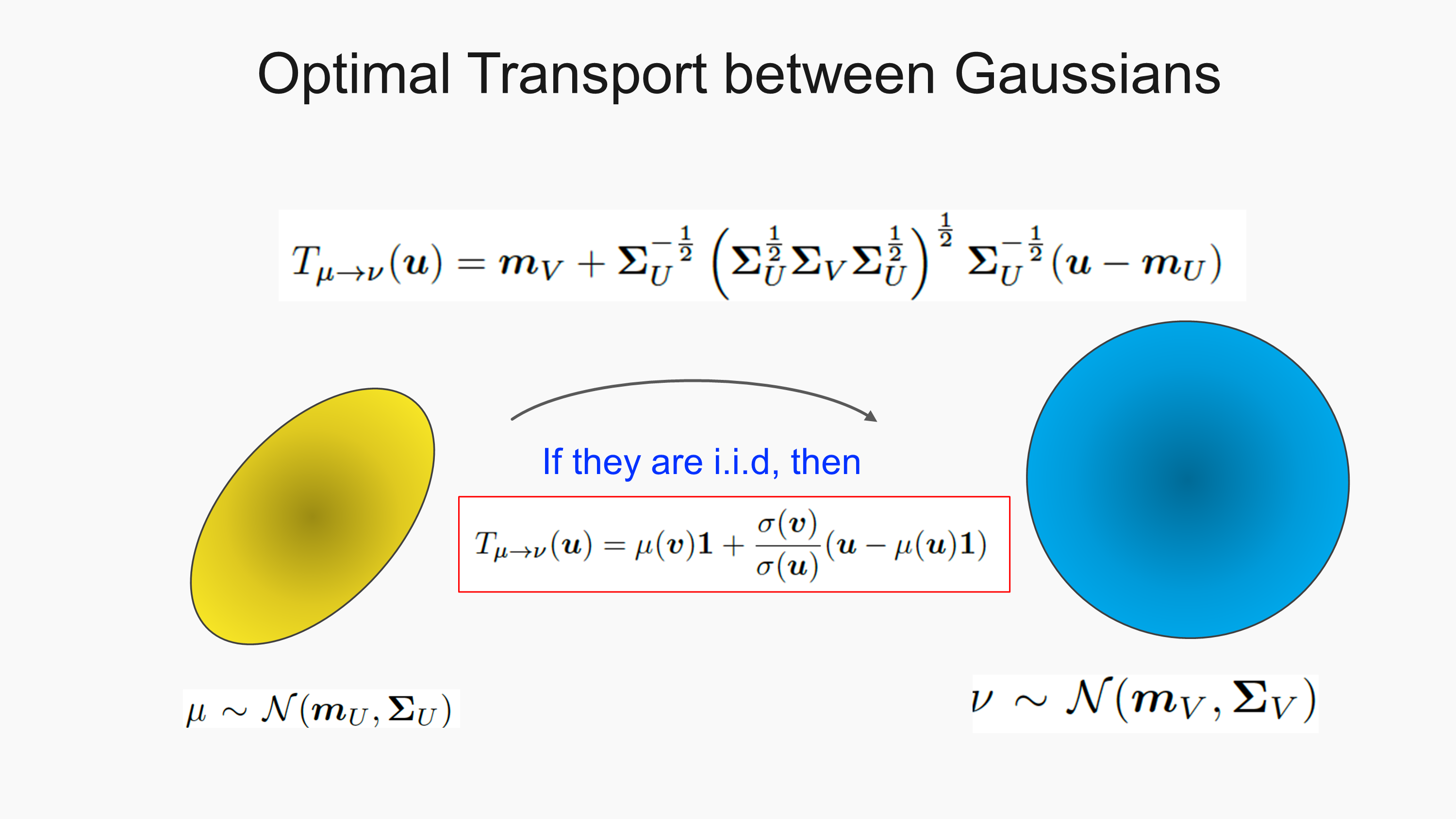
Figure 1.12 is worth keeping in view through the next two sections, because the step from the general map to the boxed one is the whole of the connection to adaptive instance normalisation: the matrix square roots collapse to a ratio of scalars the moment the covariances commute.
Proposition 1.10 (Optimal transport between Gaussians) Let \mu = \mathcal{N}(m_{U}, \Sigma_{U}) and \nu = \mathcal{N}(m_{V}, \Sigma_{V}) with \Sigma_{U} positive definite. Put
A = \Sigma_{U}^{-1/2} \bigl( \Sigma_{U}^{1/2} \Sigma_{V} \Sigma_{U}^{1/2} \bigr)^{1/2} \Sigma_{U}^{-1/2} , \qquad T_{\mu \to \nu}(u) = m_{V} + A \, (u - m_{U}) . \tag{1.34}
Then A is symmetric positive semi-definite, T_{\mu \to \nu} is the gradient of a convex function, T_{\mu \to \nu \#}\mu = \nu, and
W_{2}^{2}(\mu,\nu) = \lVert m_{U} - m_{V} \rVert^{2} + \operatorname{tr}\Bigl( \Sigma_{U} + \Sigma_{V} - 2 \bigl( \Sigma_{U}^{1/2}\Sigma_{V}\Sigma_{U}^{1/2} \bigr)^{1/2} \Bigr) . \tag{1.35}
Proof. Write S = \Sigma_{U}^{1/2}, symmetric positive definite, and M = (S \Sigma_{V} S)^{1/2}, symmetric positive semi-definite, so that A = S^{-1} M S^{-1}.
Symmetry and positivity. A^{\top} = (S^{-1})^{\top} M^{\top} (S^{-1})^{\top} = S^{-1} M S^{-1} = A, and for any z, z^{\top} A z = (S^{-1}z)^{\top} M (S^{-1}z) \geq 0.
Gradient of a convex function. Set \phi(u) = \tfrac{1}{2} u^{\top} A u + (m_{V} - A m_{U})^{\top} u. Then \nabla \phi(u) = A u + m_{V} - A m_{U} = T_{\mu \to \nu}(u), and \phi is convex because A is positive semi-definite. By Theorem 1.8 this identifies T_{\mu \to \nu} as the optimal map, provided it pushes \mu to \nu.
Push-forward. If u \sim \mathcal{N}(m_{U}, \Sigma_{U}) then T_{\mu \to \nu}(u) is Gaussian with mean m_{V} and covariance A \Sigma_{U} A. Compute, using \Sigma_{U} = S^{2} and M^{2} = S\Sigma_{V}S:
A \Sigma_{U} A = S^{-1} M S^{-1} \cdot S^{2} \cdot S^{-1} M S^{-1} = S^{-1} M^{2} S^{-1} = S^{-1} S \Sigma_{V} S S^{-1} = \Sigma_{V} .
So the push-forward is \mathcal{N}(m_{V},\Sigma_{V}) = \nu.
The distance. By Proposition 1.8 and Theorem 1.8 the optimal cost is attained at this map, so with u \sim \mu and w = u - m_{U},
\begin{aligned} W_{2}^{2}(\mu,\nu) &= \mathbb{E} \bigl\lVert u - T_{\mu \to \nu}(u) \bigr\rVert^{2} = \mathbb{E} \bigl\lVert (m_{U} - m_{V}) + (I - A) w \bigr\rVert^{2} \\ &= \lVert m_{U} - m_{V} \rVert^{2} + \operatorname{tr}\bigl( (I-A) \Sigma_{U} (I-A) \bigr) , \end{aligned}
the cross term vanishing because \mathbb{E}w = 0. Expanding the trace,
\operatorname{tr}\bigl( \Sigma_{U} - 2 A \Sigma_{U} + A \Sigma_{U} A \bigr) = \operatorname{tr}\Sigma_{U} - 2 \operatorname{tr}(A\Sigma_{U}) + \operatorname{tr}\Sigma_{V} ,
using A\Sigma_{U}A = \Sigma_{V} from above and the symmetry of A and \Sigma_{U}. Finally, by cyclicity of the trace, \operatorname{tr}(A\Sigma_{U}) = \operatorname{tr}(S^{-1}MS^{-1}S^{2}) = \operatorname{tr}(S^{-1}MS) = \operatorname{tr}(M), which is \operatorname{tr}((\Sigma_{U}^{1/2}\Sigma_{V}\Sigma_{U}^{1/2})^{1/2}). Substituting gives Equation 1.35.
Example 1.3 (The isotropic case is adaptive instance normalisation) Suppose the two Gaussians are isotropic, \Sigma_{U} = \sigma(u)^{2} I and \Sigma_{V} = \sigma(v)^{2} I. Then S = \sigma(u) I, M = (\sigma(u)^{2}\sigma(v)^{2} I)^{1/2} = \sigma(u)\sigma(v) I, and
A = \frac{1}{\sigma(u)} \cdot \sigma(u)\sigma(v) \cdot \frac{1}{\sigma(u)} I = \frac{\sigma(v)}{\sigma(u)} I ,
so Equation 1.34 becomes
T_{\mu \to \nu}(u) = \mu(v) \mathbf{1} + \frac{\sigma(v)}{\sigma(u)} \bigl( u - \mu(u) \mathbf{1} \bigr) , \tag{1.36}
writing \mu(\cdot) and \sigma(\cdot) for the scalar mean and standard deviation. Equation 1.36 is exactly the adaptive instance normalisation layer used in style transfer: standardise the content features and rescale them by the statistics of the style features. So AdaIN is not a heuristic — it is the optimal transport map between two isotropic Gaussians, and it will reappear under that name in the lecture on StyleGAN.
The Gaussian formulas are easy to get wrong by a transpose, so they are worth checking once numerically:
import numpy as np
from scipy.linalg import sqrtm

rng = np.random.default_rng(0)
d = 4
def rand_cov():
    B = rng.normal(size=(d, d))
    return B @ B.T + d * np.eye(d)

mU, mV = rng.normal(size=d), rng.normal(size=d)
SU, SV = rand_cov(), rand_cov()

S  = np.real(sqrtm(SU))
Si = np.linalg.inv(S)
M  = np.real(sqrtm(S @ SV @ S))
A  = Si @ M @ Si                                  # equation (gaussian-map)

print(np.allclose(A, A.T))                        # True: A is symmetric
print(np.linalg.eigvalsh(A).min() > 0)            # True: A is positive definite
print(np.allclose(A @ SU @ A, SV))                # True: pushes mu to nu

w2 = np.sum((mU - mV) ** 2) + np.trace(SU + SV - 2 * M)
u  = rng.multivariate_normal(mU, SU, 400_000)
t  = mV + (u - mU) @ A.T                          # A symmetric, so A.T == A
print(w2, np.mean(np.sum((u - t) ** 2, axis=1)))  # the two agree
1.14 Back to generative models
We can now close the loop opened in Section 1.3. A generator defines \mu_{\theta} = G_{\theta \#}\nu by Equation 1.1, and training means minimising some discrepancy D(\mu_{\theta}, p_{\text{data}}) over \theta. This chapter has supplied two families of candidates for D, and the choice between them is an optimisation decision rather than a matter of taste.
Take D to be an f-divergence and one obtains the adversarial models. The original GAN objective, at its optimal discriminator, reduces to the Jensen–Shannon divergence between \mu_{\theta} and p_{\text{data}} up to an additive constant; f-GAN generalises this by replacing the generator f and deriving the corresponding variational bound. Theorem 1.2 is then the warning label on the whole construction: as soon as the discriminator becomes good enough to separate the two supports, the objective is pinned at f(0) + f'(\infty) and its gradient in \theta vanishes.
Take D to be an integral probability metric and one obtains the alternatives. W-GAN takes \mathcal{F} = \mathrm{Lip}_{1} and optimises the dual in Equation 1.32, which is why its critic is Lipschitz-constrained and why its loss remains informative when the supports are disjoint — by Example 1.1 it still reports \lvert \theta \rvert. The general statement behind that example — that the loss is continuous in \theta, where the Jensen–Shannon one is not — is Section 1.15.10. McGAN and MMD-GAN take \mathcal{F} to be a moment class or an RKHS ball and use Equation 1.20, which is estimable directly from two samples and needs no inner maximisation at all.
| Discrepancy | Metric | Needs P \ll Q | Value when P \perp Q | Used by |
|---|---|---|---|---|
| D_{\mathrm{KL}} | no | yes | +\infty | maximum likelihood |
| Reverse D_{\mathrm{KL}} | no | yes | +\infty | variational inference |
| D_{\mathrm{JS}} | no | no | \log 2 | GAN, f-GAN |
| Total variation | yes | no | 1 | analysis, rarely trained |
| \mathrm{MMD} | yes | no | varies with the kernel | MMD-GAN, McGAN |
| W_{1} | yes | no | varies with the distance | W-GAN |
The last two rows are the point of the table. Only for the integral probability metrics does the entry in the fourth column depend on the configuration of the two distributions rather than on the discrepancy alone, and that dependence is precisely the gradient signal a generator needs. Figure 1.13 collects the whole development onto one page.
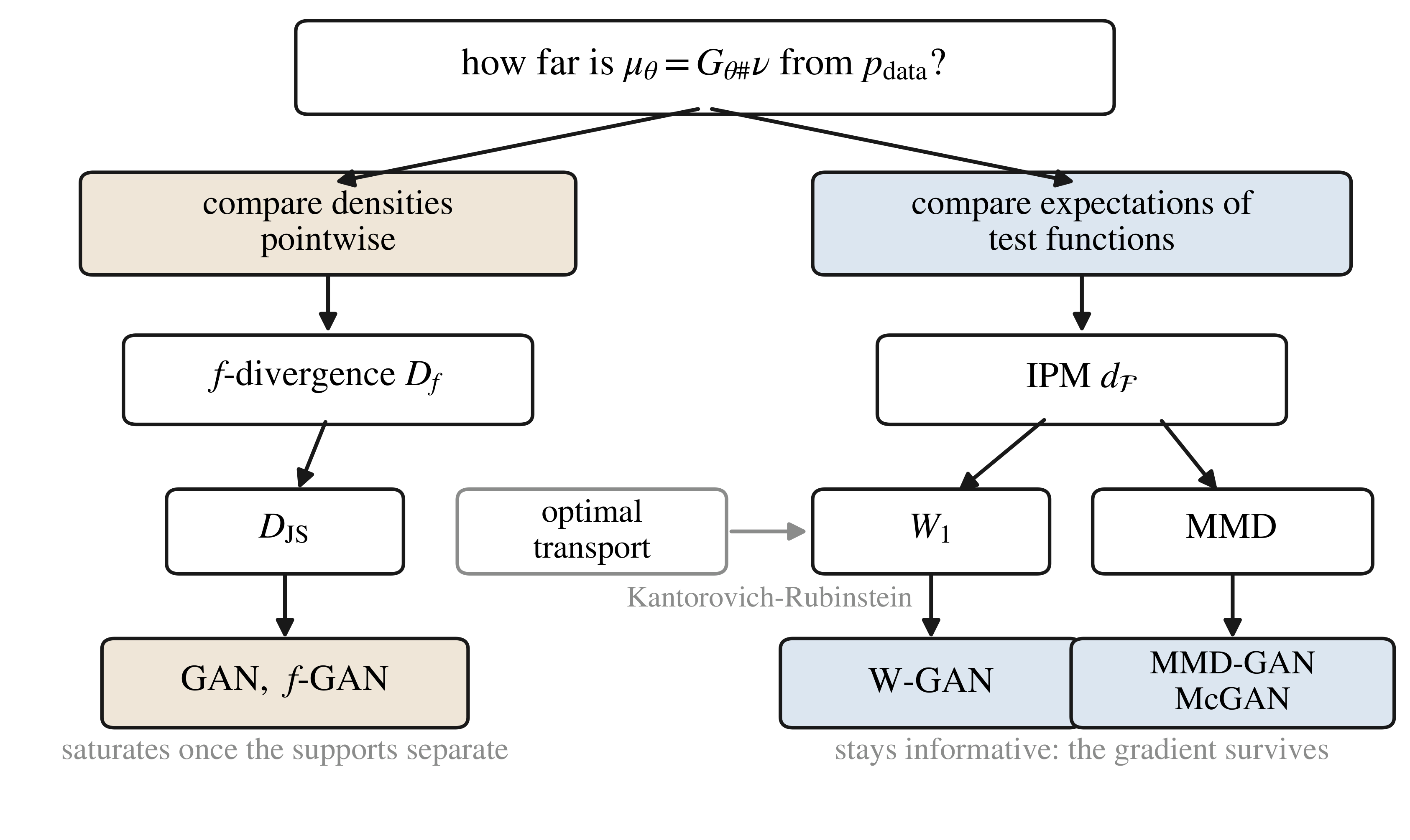
Three threads continue directly into the next lectures. The reduction of the GAN objective to the Jensen–Shannon divergence, and the f-GAN variational bound, are the subject of Lecture 02, as are W-GAN, McGAN and the geometric view. Equation 1.36, the optimal map between isotropic Gaussians, returns as the adaptive instance normalisation layer of StyleGAN in Lecture 03. And the idea that a generative model is a transport of one measure onto another — rather than a likelihood to be maximised — is the thread that runs through the diffusion, flow matching and Schrodinger bridge lectures in the rest of the course.
1.15 Advanced topics
The chapter above follows the lecture. This section collects material that the lecture did not cover but that the development above leans on or leaves open: a divergence the tables list without evaluating, the two estimators that make the maximum mean discrepancy usable, the linear-programming form of the Kantorovich problem, the hypotheses under which duality survives the passage to Polish spaces, and the topological facts that turn Example 1.1 from an example into a theorem about training. Each subsection is self-contained and none is needed to follow the main line.
1.15.1 Where the Pearson chi-squared divergence is finite
The generator table of Section 1.6 lists f(u) = (u-1)^{2}, and the saturation table of Section 1.7 gives its row, but neither is worked through in the chapter. Here f(0) = 1 and f'(\infty) = \lim_{u \to \infty} (u-1)^{2}/u = +\infty, so by Theorem 1.2 the Pearson \chi^{2} divergence is +\infty on mutually singular pairs, joining the two Kullback–Leibler divergences rather than the bounded generators.
Away from that case,
D_{\chi^{2}}(P \Vert Q) = \int \left( \frac{dP}{dQ} - 1 \right)^{2} dQ = \int \left( \frac{dP}{dQ} \right)^{2} dQ \; - \; 1 , \tag{1.37}
so \chi^{2} is finite exactly when P \ll Q and dP/dQ \in L^{2}(Q). That is a strictly stronger demand than the absolute continuity D_{\mathrm{KL}} needs, and it is why \chi^{2} plays no part in the generative models of this course: the situation of Section 1.7 defeats it even more thoroughly than the others.
1.15.2 How literal is the dual-norm reading?
Definition 1.8 was introduced as the norm of the signed measure \mu - \nu measured over a unit ball. The reading is exact for two of the three classes of Section 1.8 and only approximate for the third, and the difference is worth pinning down because it is the reason Theorem 1.7 needs a normalisation.
If \lVert \cdot \rVert_{B} is a genuine norm on a space B of test functions and \mathcal{F} = \{ h : \lVert h \rVert_{B} \leq 1 \}, then
d_{\mathcal{F}}(\mu,\nu) = \lVert \mu - \nu \rVert_{B^{\ast}} \tag{1.38}
by the definition of the dual norm. The indicator class and the RKHS ball of Proposition 1.6 are of this kind. The class \mathrm{Lip}_{1} is not: the Lipschitz constant vanishes on constant functions, so it is a seminorm rather than a norm, and \mathrm{Lip}_{1} is unbounded in any function norm — it contains \varphi + t for every real t. The dual reading is recovered by quotienting out the constants, which is legitimate here because \mu - \nu annihilates them, both measures having total mass 1; equivalently, by normalising \varphi(x_{0}) = 0 at a base point, which is what one does in practice when implementing Equation 1.32.
The choice of \mathcal{F} also fixes a topology on \mathcal{P}(\mathcal{X}), and the three are genuinely different:
| \mathcal{F} | Metric | Topology induced |
|---|---|---|
| indicators \mathbf{1}_{A} | total variation | strictly finer than weak; the one Theorem 1.2 bites in |
| \{ h : \lVert h \rVert_{\infty} + \mathrm{Lip}(h) \leq 1 \} | bounded-Lipschitz | weak convergence |
| \mathrm{Lip}_{1} | W_{1} | weak convergence, on a space of bounded diameter |
The second row is the Dudley metric. The third is what Section 1.15.4 takes up in general, and the gap between the first row and the other two is the whole argument of Section 1.14.
1.15.3 Estimating the maximum mean discrepancy
Equation 1.20 writes \mathrm{MMD}^{2} entirely in terms of expectations of the kernel, which is what makes it usable: no density estimate and no inner maximisation. Given x_{1},\dots,x_{m} \sim \mu and y_{1},\dots,y_{n} \sim \nu independently, replacing each expectation by the corresponding sample average gives the V-statistic
\widehat{\mathrm{MMD}}^{2}_{V} = \frac{1}{m^{2}} \sum_{i,j} k(x_{i},x_{j}) - \frac{2}{mn} \sum_{i,j} k(x_{i},y_{j}) + \frac{1}{n^{2}} \sum_{i,j} k(y_{i},y_{j}) . \tag{1.39}
It is biased upwards, because the diagonal terms k(x_{i},x_{i}) estimate \mathbb{E}_{x,x'}k(x,x') with x' = x rather than with an independent copy. Deleting the diagonals gives the U-statistic
\widehat{\mathrm{MMD}}^{2}_{U} = \frac{1}{m(m-1)} \sum_{i \neq j} k(x_{i},x_{j}) - \frac{2}{mn} \sum_{i,j} k(x_{i},y_{j}) + \frac{1}{n(n-1)} \sum_{i \neq j} k(y_{i},y_{j}) , \tag{1.40}
which is unbiased for \mathrm{MMD}^{2} but is no longer a squared norm, so a single estimate can come out negative when the two distributions agree. Both need O\bigl((m+n)^{2}\bigr) kernel evaluations. That quadratic cost is what keeps the maximum mean discrepancy to moderate batch sizes, and is the practical reason it is more often used as a two-sample test statistic than as a training loss at scale.
Whether the maximum mean discrepancy separates distributions at all is a property of the kernel and not of the estimator. Call k characteristic if the mean embedding \mu \mapsto m_{\mu} is injective on \mathcal{P}(\mathcal{X}); by Proposition 1.5 this is exactly the condition under which \mathrm{MMD}(\mu,\nu) = 0 if and only if \mu = \nu, that is, under which Equation 1.19 is a metric and not merely a pseudo-metric. For a translation-invariant kernel on \mathbb{R}^{d} the condition can be read off the spectrum. Bochner’s theorem writes
k(x,y) = \int_{\mathbb{R}^{d}} e^{i \langle \omega, \, x-y \rangle} \, d\Lambda(\omega) \tag{1.41}
for a finite non-negative spectral measure \Lambda, and k is characteristic exactly when \mathrm{supp}(\Lambda) = \mathbb{R}^{d}: the embedding then sees every frequency of the characteristic function of \mu - \nu, so no non-zero difference can be invisible. The Gaussian kernel qualifies, its spectral measure being Gaussian and hence of full support. A band-limited kernel does not, and is blind to whatever the two distributions do above its cutoff.
1.15.4 The topology of the Wasserstein distance
Theorem 1.3 establishes that W_{p} is a metric. That alone is not the property Section 1.14 relies on; what matters is which notion of convergence it defines. On a Polish space,
W_{p}(\mu_{n},\mu) \to 0 \iff \mu_{n} \to \mu \ \text{weakly} \ \ \text{and} \ \ \int d(x,x_{0})^{p} d\mu_{n} \to \int d(x,x_{0})^{p} d\mu \tag{1.42}
for some — equivalently any — base point x_{0}. On a space of bounded diameter, which is the case for images confined to a fixed pixel range, the moment condition is automatic and W_{p} metrises weak convergence outright.
No f-divergence does this. Total variation and the Jensen–Shannon divergence induce a strictly finer topology, and Example 1.1 is the gap made concrete: \mu_{\theta} \to \mu_{0} weakly as \theta \to 0, yet both stay pinned at their saturation values until the instant \theta = 0. That mismatch of topologies, rather than the arithmetic of any single example, is the precise sense in which the Wasserstein distance “still varies smoothly” where the others do not, and Section 1.15.10 turns it into a statement about training.
1.15.5 Two further ways Monge’s problem fails
Proposition 1.7 rules out a transport map by an atom: a map cannot split mass. It is easy to read that as the only difficulty, and to conclude that a non-atomic \mu makes Equation 1.24 well behaved. It does not. The feasible set \{T : T_{\#}\mu = \nu\} is not closed in any topology for which \mathbb{M} is continuous, so the infimum can fail to be attained even when feasible maps are plentiful.
Example 1.4 (An infimum with no minimiser) Work in \mathbb{R}^{2} with c(x,y) = \lVert x-y \rVert. Let \mu be uniform on the segment \{0\} \times [0,1], and let \nu = \tfrac{1}{2}\nu_{-} + \tfrac{1}{2}\nu_{+} with \nu_{\pm} uniform on \{\pm 1\} \times [0,1]. Then \inf_{T} \mathbb{M}(T) = 1, but \mathbb{M}(T) > 1 for every feasible T, so no optimal map exists.
Proof. Every feasible map costs more than 1. A point x = (0,t) and a point y = (\pm 1, s) of the target are at distance \sqrt{1 + (t-s)^{2}} \geq 1, with equality only when s = t. So \mathbb{M}(T) \geq 1 always, with equality only if T preserves height \mu-almost everywhere. But a height-preserving T pushes \mu onto a set meeting each height at most once, whereas \nu charges two points at every height; such a T is not feasible. Hence \mathbb{M}(T) > 1.
The infimum is 1. Cut [0,1] into 2n strips of height 1/(2n) and let T_{n} send the odd strips to the left target and the even strips to the right, each by the affine map onto the corresponding strip of height 1/n. Each half receives mass n \cdot \tfrac{1}{2n} = \tfrac{1}{2} spread uniformly, so T_{n} is feasible, and it moves any point vertically by at most 1/n, so \mathbb{M}(T_{n}) \leq \sqrt{1 + n^{-2}} \to 1.
Kantorovich attains it. The plan that splits each (0,t) evenly between (-1,t) and (1,t) is a coupling of cost exactly 1.
This example also sharpens Equation 1.27: there the inequality is strict with both sides finite, which Proposition 1.7, whose right-hand side is an infimum over the empty set, could not show.
Failure of uniqueness is a third phenomenon, independent of the other two. For Monge’s original cost c(x,y) = \lVert x-y \rVert, take \mu = \mathrm{Uniform}[0,1] and \nu = \mathrm{Uniform}[2,3] on the line. Every target point lies to the right of every source point, so \lvert x-y \rvert = y-x and every feasible map has the same cost \mathbb{E}_{\nu}[y] - \mathbb{E}_{\mu}[x] = 2. All of them are optimal, including the monotone map of Theorem 1.4 and including maps that reverse order. Uniqueness, when it holds, comes from strict convexity of the cost — it is the quadratic cost of Theorem 1.8 that forces a single answer, not transport as such.
1.15.6 The Kantorovich problem as a linear program
On finite spaces Equation 1.26 is a linear program, and it is worth displaying rather than leaving inside the proof of Theorem 1.6: it is what a solver actually receives, and its shape is the reason the dual of Section 1.12, and not the primal, is what generative models implement. Take \mathcal{X} = \{x_{1},\dots,x_{m}\} and \mathcal{Y} = \{y_{1},\dots,y_{n}\}, collect the marginals into vectors \mu \in \mathbb{R}^{m} and \nu \in \mathbb{R}^{n} and the costs into the matrix C_{ij} = c(x_{i},y_{j}). A coupling is a matrix \Pi \in \mathbb{R}^{m \times n} and Equation 1.26 reads
\min_{\Pi \geq 0} \; \langle C, \Pi \rangle = \sum_{i,j} C_{ij}\Pi_{ij} \qquad \text{subject to} \qquad \Pi \mathbf{1}_{n} = \mu , \quad \Pi^{\top} \mathbf{1}_{m} = \nu . \tag{1.43}
The feasible set of Equation 1.43 is the transportation polytope of \mu and \nu: non-empty, compact and convex. It carries mn non-negative variables against only m+n equality constraints, one of which is redundant, since summing either family returns the total mass 1; so m+n-1 are independent. That imbalance is the whole of computational optimal transport. The primal holds a variable for every pair of points, the dual of Section 1.12 one per point, and once m and n reach the tens of thousands only the second can be stored at all.
The polytope also settles when Monge and Kantorovich agree. Suppose m = n and both marginals are uniform, \mu = \nu = \tfrac{1}{n}\mathbf{1}_{n}. The feasible set is then \tfrac{1}{n}\mathcal{B}_{n}, where \mathcal{B}_{n} is the Birkhoff polytope of doubly stochastic matrices. By the Birkhoff–von Neumann theorem the extreme points of \mathcal{B}_{n} are exactly the permutation matrices, and a linear objective on a compact convex polytope attains its minimum at an extreme point. So an optimal plan may be taken to be \tfrac{1}{n}P_{\sigma} for a permutation \sigma — that is, to be induced by a map after all, and Equation 1.27 holds with equality. The relaxation costs nothing for discrete measures with equal atom weights; it earns its keep in the unequal and continuous cases, which are the ones Proposition 1.7 and Example 1.4 describe.
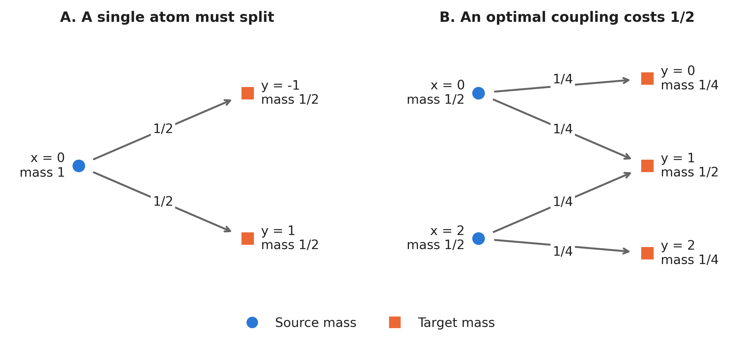
1.15.7 Duality beyond finite spaces
The proof of Theorem 1.6 settles strong duality on finite spaces and defers the rest to a citation. Two things that citation hides are worth stating; a consequence for the optimal plans themselves follows in Section 1.15.8.
What the general theorem needs. Strong duality in Equation 1.29 holds whenever \mathcal{X} and \mathcal{Y} are Polish and c is lower semicontinuous and bounded below. Neither continuity of c nor finiteness of the optimal value is required. The proof is not a limit of the finite argument above; it is a Fenchel–Rockafellar duality in the pair \bigl( C_{b}(\mathcal{X} \times \mathcal{Y}), \mathcal{M}(\mathcal{X} \times \mathcal{Y}) \bigr), with the lower semicontinuous c approached from below by bounded continuous costs.
When the supremum is attained. Equation 1.29 is written with a supremum and not a maximum deliberately: optimal potentials need not exist. They do exist, and are then called Kantorovich potentials as in Definition 1.14, under a mild domination hypothesis — it is enough that c be continuous and that c(x,y) \leq a(x) + b(y) for some a \in L^{1}(\mu) and b \in L^{1}(\nu). Both costs used in this chapter satisfy it whenever the measures have the moments Definition 1.10 assumes, since \lVert x-y \rVert \leq \lVert x \rVert + \lVert y \rVert and \tfrac{1}{2}\lVert x-y \rVert^{2} \leq \lVert x \rVert^{2} + \lVert y \rVert^{2}. This is the hypothesis that licenses Theorem 1.8 to begin by taking optimal potentials as given.
1.15.8 Complementary slackness and cyclical monotonicity
Duality constrains the optimal plans themselves and not only the optimal value. The weak-duality computation in Theorem 1.6 integrated an inequality; once the two optimal values agree, that inequality has nowhere left to hide.
Proposition 1.11 (Complementary slackness) Let \pi be optimal for Equation 1.26 and (\varphi,\psi) optimal for Equation 1.29, with the common value finite. Then
\varphi(x) + \psi(y) = c(x,y) \qquad \text{for } \pi\text{-almost every } (x,y) , \tag{1.44}
so \pi is concentrated on the set where the dual constraint is active. When \psi = \varphi^{c}, that set is the c-superdifferential of \varphi.
Proof. The function c(x,y) - \varphi(x) - \psi(y) is non-negative by the definition of \Phi_{c}, and its integral against \pi is \mathbb{K}(\pi) - \mathbb{J}(\varphi,\psi), which vanishes by Equation 1.29. A non-negative function with zero integral is zero almost everywhere.
Equation 1.44 is the engine of every structural result about optimal plans; it is what Theorem 1.8 uses to turn a coupling into a map. It also has a consequence that mentions no potentials at all. If \pi is optimal then \mathrm{supp}(\pi) is c-cyclically monotone: for every finite family (x_{1},y_{1}),\dots,(x_{N},y_{N}) in the support and every permutation \sigma of \{1,\dots,N\},
\sum_{i=1}^{N} c(x_{i},y_{i}) \; \leq \; \sum_{i=1}^{N} c\bigl( x_{i}, y_{\sigma(i)} \bigr) . \tag{1.45}
The proof is one line from Equation 1.44: summing the equality over the family gives \sum_{i} c(x_{i},y_{i}) = \sum_{i}\varphi(x_{i}) + \sum_{i}\psi(y_{i}), the right-hand side is unchanged by reindexing \psi along \sigma, and \varphi(x_{i}) + \psi(y_{\sigma(i)}) \leq c(x_{i},y_{\sigma(i)}) term by term. In words: no finite reshuffling of destinations among the pairs the plan actually uses can lower the bill. For c continuous and real-valued the converse holds as well — a coupling with c-cyclically monotone support is optimal — so Equation 1.45 characterises optimality with no reference to the dual problem.
1.15.9 The c-transform for the quadratic cost
For c(x,y) = \lVert x-y \rVert the c-transform of a 1-Lipschitz function is simply its negative, which is Lemma 1.3. For the quadratic cost it is the Legendre transform wearing a disguise, and that identification is the whole of the change of variables in Theorem 1.8.
c(x,y) = \tfrac{1}{2}\lVert x-y \rVert^{2} the c-transform is the Legendre transform wearing a disguise. Put u(x) = \tfrac{1}{2}\lVert x \rVert^{2} - \varphi(x) and expand the square:
\varphi^{c}(y) = \inf_{x} \Bigl\{ \tfrac{1}{2}\lVert x-y \rVert^{2} - \varphi(x) \Bigr\} = \tfrac{1}{2}\lVert y \rVert^{2} - \sup_{x} \bigl\{ \langle x,y \rangle - u(x) \bigr\} = \tfrac{1}{2}\lVert y \rVert^{2} - u^{\ast}(y) . \tag{1.46}
So \varphi is c-concave for the quadratic cost exactly when u = \tfrac{1}{2}\lVert \cdot \rVert^{2} - \varphi is convex and lower semicontinuous: applying Equation 1.46 twice turns c-concavity of \varphi into the identity u = u^{\ast\ast}, which is the Fenchel–Moreau theorem. It is worth registering that what appears is convexity of u and not concavity — the c-transform reverses order, and the \tfrac{1}{2}\lVert \cdot \rVert^{2} absorbs the sign. This identification is the entire change of variables of Theorem 1.8, which carries it out in a single line.
1.15.10 Continuity of the Wasserstein loss
Example 1.1 shows one generator, with one parameter, on which W_{1} carries a gradient and the f-divergences do not. The general statement rests on Section 1.15.4: W_{1} metrises weak convergence on a space of bounded diameter, whereas total variation and the Jensen–Shannon divergence induce a strictly finer topology.
Suppose G_{\theta}(z) is locally Lipschitz in \theta, uniformly in z up to an integrable envelope — a condition any feed-forward network with Lipschitz activations satisfies. Then \theta \mapsto \mu_{\theta} is continuous for weak convergence, so by Equation 1.42
\theta \mapsto W_{1}(\mu_{\theta}, p_{\text{data}}) \tag{1.47}
is continuous everywhere and, being locally Lipschitz, differentiable almost everywhere. Gradient descent on it is therefore well posed wherever it is run.
No such statement is available for D_{\mathrm{JS}}. By Theorem 1.2 it is locally constant wherever the supports separate, which by the dimension count of Section 1.7 is essentially everywhere; it is differentiable almost everywhere too, but with derivative zero, which is worse than useless. This is Theorem 1 of Arjovsky, Chintala and Bottou, and it is the reason the loss was worth changing.
1.16 Appendix: proof of the Radon–Nikodym theorem
Theorem 1.1 was used throughout without proof. The following argument, due to von Neumann, is short and uses only the Riesz representation theorem in a Hilbert space, so it is worth including rather than citing.
Proof. Assume first that \lambda and \nu are finite, with \lambda \ll \nu, and set \rho = \lambda + \nu, also finite. Consider the linear functional
L(f) = \int_{\Omega} f \, d\lambda , \qquad f \in L^{2}(\rho) .
It is bounded: by Cauchy–Schwarz in L^{2}(\rho), and since \lambda \leq \rho,
\lvert L(f) \rvert \leq \int \lvert f \rvert \, d\lambda \leq \int \lvert f \rvert \, d\rho \leq \lVert f \rVert_{L^{2}(\rho)} \, \rho(\Omega)^{1/2} .
By the Riesz representation theorem there is g \in L^{2}(\rho) with
\int f \, d\lambda = \int f g \, d\rho = \int f g \, d\lambda + \int f g \, d\nu \qquad \text{for all } f \in L^{2}(\rho) ,
and rearranging,
\int f \, (1 - g) \, d\lambda = \int f g \, d\nu . \tag{1.48}
Taking f = \mathbf{1}_{\{g < 0\}} in \int f d\lambda = \int fg \, d\rho forces \rho(\{g<0\}) = 0, and taking f = \mathbf{1}_{\{g>1\}} gives \int_{\{g>1\}} (1-g) \, d\lambda = \int_{\{g>1\}} g \, d\nu \geq 0 with a strictly negative left-hand side unless \rho(\{g>1\}) = 0. So 0 \leq g \leq 1 \rho-almost everywhere.
Let N = \{ g = 1 \}. Taking f = \mathbf{1}_{N} in Equation 1.48 gives 0 = \nu(N), and since \lambda \ll \nu also \lambda(N) = 0.
Now fix a measurable A and take f = \mathbf{1}_{A}\bigl( 1 + g + \cdots + g^{n-1} \bigr) in Equation 1.48. The left-hand side telescopes, since (1 + \cdots + g^{n-1})(1-g) = 1 - g^{n}:
\int_{A} \bigl( 1 - g^{n} \bigr) d\lambda = \int_{A} \bigl( g + g^{2} + \cdots + g^{n} \bigr) d\nu .
Let n \to \infty. On \{g < 1\} we have g^{n} \to 0, and \lambda(N) = 0, so the left side tends to \lambda(A) by dominated convergence. The right side increases to \int_{A} \sum_{k \geq 1} g^{k} \, d\nu = \int_{A} \frac{g}{1-g} \, d\nu by monotone convergence, the integrand being defined \nu-almost everywhere because \nu(N) = 0. Hence
\lambda(A) = \int_{A} h \, d\nu , \qquad h = \frac{g}{1-g} \geq 0 ,
which is Equation 1.3. For \sigma-finite measures, partition \Omega into countably many sets of finite measure and add the resulting densities.
Uniqueness: if \int_{A} h_{1} d\nu = \int_{A} h_{2} d\nu for every A, then taking A = \{h_{1} > h_{2}\} and A = \{h_{1} < h_{2}\} in turn forces both sets to be \nu-null, so h_{1} = h_{2} \nu-almost everywhere.
1.17 Further reading
Full bibliographic details are on the book’s References page. The lecture follows Chapters 1 and 13 of the course text; the transport material beyond it is standard and the sources below are where each statement used here is proved in full.
- Ye (2022) — Chapter 1 for metric spaces, convexity and duality; Chapter 13 for statistical distances and optimal transport. Definitions and equation numbers quoted in this chapter follow that text.
- Villani (2003) — Theorem 1.3 is the general form of Theorem 1.6; Chapter 1 covers the c-transform and c-concavity.
- Villani (2009) — Chapter 5 for duality, Chapter 6 for the metric structure of W_{p} and the gluing lemma.
- Santambrogio (2015) — Theorem 2.9 proves that the monotone map is optimal for costs h(x-y) with h convex, which Theorem 1.4 cites.
- Peyré and Cuturi (2019) — the linear-programming view of Definition 1.13 and its numerics.
- Brenier (1991) — the original form of Theorem 1.8.
- McCann (1995) — removes the moment hypotheses from Brenier’s theorem.
- Csiszár (1967) — the origin of Definition 1.6.
- Sriperumbudur et al. (2009) — proves that total variation is the only non-trivial member of both families, the claim made in Section 1.8.
- Gretton et al. (2012) — the source for Proposition 1.6 and for characteristic kernels.
- Goodfellow et al. (2014) — the original adversarial formulation.
- Nowozin et al. (2016) — Table 2 there lists the generators in the convention discussed after Proposition 1.4.
- Arjovsky and Bottou (2017) — the manifold argument of Section 1.7.
- Arjovsky et al. (2017) — Example 1 there is Example 1.1.
- Mroueh et al. (2017) — mean and covariance feature matching.
- Huang and Belongie (2017) — the layer identified with Equation 1.36.
Based on the scribe note of Jungwoo Ahn, with material from Sungwon Yang and Junhyeong Park; edited by Jong Chul Ye.