6 Denoising Diffusion Probabilistic Models
6.1 Overview
A diffusion model splits the hard problem of sampling from a complex data distribution into two parts: an easy forward process that adds a little Gaussian noise many times, and a learned reverse process that undoes it. The forward process is fixed. It gradually erases the structure of the data until the state is close to a standard Gaussian. The reverse process starts from noise and is trained, as a neural network, to remove a little noise at every step (Ho et al. 2020).
This chapter develops that construction from first principles, following slides 2–25 of the lecture deck Diffusion Model Theory (Ye 2026): the DDPM derivation on slides 2–16 and DDIM on slides 17–25. It begins with the probability tools needed to describe a latent Markov chain, derives the closed-form forward marginal and the variational training objective, and then turns the resulting Gaussian mean-matching problem into noise prediction. The relation among noise, data and velocity prediction makes the role of the loss weighting explicit. Finally, ancestral DDPM sampling is compared with the non-Markovian inference family and deterministic sampling rule of DDIM (Sohl-Dickstein et al. 2015; Ho et al. 2020; J. Song et al. 2021).
The construction rests on three mathematical facts.
- Even after many Markov Gaussian transitions, x_t at any time can be sampled from x_0 in a single step, in closed form.
- Fitting the intractable reverse conditionals becomes, through a variational bound, a sum of Gaussian KL divergences that can be computed.
- Predicting the noise \epsilon that the forward process added, instead of the reverse mean, turns each term of the objective into a weighted mean squared error, which DDPM then simplifies to a plain one.
The exact reverse conditional is generally not Gaussian, but it becomes locally close to Gaussian when each forward step is small. This motivates the many-step DDPM construction. DDIM instead changes the inference path while preserving the same noisy marginals, which permits deterministic and shortened sampling trajectories (Ho et al. 2020; J. Song et al. 2021). Short proofs follow the results they prove; longer verifications are collected in the appendix (Section 6.9).
After reading this note you should be able to:
- derive the closed form of q(x_t\mid x_0) from q(x_t\mid x_{t-1});
- decompose the variational bound on the negative log-likelihood into L_T, L_{t-1} and L_0;
- compute the mean and variance of q(x_{t-1}\mid x_t,x_0) by completing the square;
- show that mean prediction and noise prediction describe the same reverse mean, and derive the noise-estimation loss;
- reproduce the DDPM training and ancestral sampling algorithms, and explain why sampling adds noise back;
- explain what it means that the non-Markovian forward process of DDIM has the same marginals as DDPM.
6.2 Notation
We follow the notation of the slides (Ye 2026), which for DDPM is that of Ho et al. (2020), except that vectors are written without boldface: x_t, \epsilon and \mu_\theta. References of the form “slide 12” point to that deck, so that each section can be checked against the lecture. The symbols are collected in Table 6.1.
| Symbol | Meaning |
|---|---|
| x_0\sim q_{\mathrm{data}} | clean sample from the data distribution, x_0\in\mathbb R^d |
| x_t, x_{a:b} | latent at noise level t (t=1,\ldots,T); x_{a:b}:=(x_a,\ldots,x_b) |
| \beta_t\in(0,1) | variance of the noise added at step t |
| \alpha_t:=1-\beta_t | fraction of the signal kept in one step (in variance) |
| \bar\alpha_t:=\prod_{s=1}^{t}\alpha_s, \bar\alpha_0:=1 | signal fraction accumulated from time 0 to t |
| a_t:=\sqrt{\bar\alpha_t}, b_t:=\sqrt{1-\bar\alpha_t} | signal and noise coefficients in x_t=a_tx_0+b_t\epsilon |
| \mathrm{SNR}(t):=\bar\alpha_t/(1-\bar\alpha_t) | signal-to-noise ratio at time t |
| \epsilon_t, z\sim\mathcal N(0,I) | noise of forward step t, and fresh noise of a sampling step; mutually independent |
| \epsilon\sim\mathcal N(0,I), \bar\epsilon_t | noise of the one-step form x_t=a_tx_0+b_t\epsilon (written \bar\epsilon_t when its time matters); independent of x_0, but along one path a function of \epsilon_1,\ldots,\epsilon_t |
| q, q_t, q_\gamma | fixed forward diffusion, its marginal q_t(x_t) at time t, and the DDIM family |
| p_\theta | reverse generative model to be learned |
| \tilde\mu_t,\tilde\beta_t | mean and variance of the exact forward posterior q(x_{t-1}\mid x_t,x_0) |
| \mu_\theta,\epsilon_\theta,\hat x_0 | reverse mean, noise prediction, and the data prediction computed from it |
| \Sigma_\theta, s_\theta | covariance of the reverse transition, and the score estimate -\epsilon_\theta/\sqrt{1-\bar\alpha_t} |
| \sigma_t^2 | variance of the DDPM reverse transition |
| w_t | coefficient of the noise-prediction MSE at time t in the variational bound |
| \gamma_t^2 (t\ge2), \gamma_1^2 | posterior variance of the DDIM family q_\gamma; \gamma_1^2>0 is the variance of its decoder p_\theta(x_0\mid x_1) |
| \eta | interpolation between DDIM (\eta=0) and DDPM (\eta=1) through \gamma_t=\eta\sqrt{\tilde\beta_t} |
| v, \phi_t | velocity target, and the angle with a_t=\cos\phi_t, b_t=\sin\phi_t |
| \mathcal N(x;m,\Sigma) | density at x of a Gaussian with mean m and covariance \Sigma |
Norms are Euclidean unless stated otherwise. \mathbb E_q denotes expectation over x_0\sim q_{\mathrm{data}} and all latents generated by the forward diffusion.
6.3 Background: the Markov property and Gaussian tools
The derivation uses the KL divergence, Jensen’s inequality and the evidence lower bound of a latent-variable model, which Section 1.6 and Section 4.3 develop. It also uses the Markov property and a few Gaussian identities, which this section states before they are applied.
6.3.1 Latent paths and the Markov factorization
The observed datum is a single x_0, but a diffusion model introduces latents x_1,\ldots,x_T at increasing noise levels, so its likelihood p_\theta(x_0)=\int p_\theta(x_{0:T})\,dx_{1:T} is bounded as for the variational autoencoder of Chapter 4, with two differences: the latent is a whole diffusion path rather than a single code, and the “encoder” q(x_{1:T}\mid x_0) is fixed rather than learned (Kingma and Welling 2014; Ho et al. 2020).
Definition 6.1 (First-order Markov chain) A sequence x_0,x_1,\ldots,x_T is a first-order Markov chain if for all t=1,\ldots,T
q(x_t\mid x_{0:t-1}) =q(x_t\mid x_{t-1}). \tag{6.1}
Equivalently, x_t\mathrel{\perp\!\!\!\perp}x_{0:t-2}\mid x_{t-1}.
Substituting Equation 6.1 into the chain rule gives q(x_{1:T}\mid x_0)=\prod_{t=1}^{T}q(x_t\mid x_{0:t-1})=\prod_{t=1}^{T}q(x_t\mid x_{t-1}). This factorization defines the forward path distribution used below.
Proposition 6.1 (A Markov chain read backwards is still Markov) If the forward chain is Markov, then q(x_{t-1}\mid x_{t:T})=q(x_{t-1}\mid x_t) for all t. Proof in Section 6.9.2.
The Markov property of the reverse chain holds whatever the step size. What needs small steps is the approximation that the reverse transition q(x_{t-1}\mid x_t) has a Gaussian functional form, which is discussed with the reverse process.
6.3.2 Chapman–Kolmogorov composition and marginals
Integrating out intermediate states composes several transitions:
q(x_t\mid x_0) =\int q(x_t\mid x_{t-1})q(x_{t-1}\mid x_0)\,dx_{t-1}. \tag{6.2}
The first factor can be written q(x_t\mid x_{t-1}) instead of q(x_t\mid x_{t-1},x_0) because of the Markov property. In DDPM both factors are linear Gaussian, so the integral is Gaussian too.
It is important to distinguish the joint distribution of a path from the marginal at one time. The product of Markov transitions fixes how the whole path is coupled, but knowing only q(x_t\mid x_0) does not determine the coupling between different times. DDIM uses exactly this freedom: it keeps the same q(x_t\mid x_0) as DDPM while using a non-Markovian path (Section 6.5) (J. Song et al. 2021).
6.3.3 Gaussian tools
Every closed form in this chapter follows from three lemmas. Their proofs are in Section 6.9.1.
Lemma 6.1 (Linear combinations of independent Gaussians) If u\sim\mathcal N(m_u,\Sigma_u) and v\sim\mathcal N(m_v,\Sigma_v) are independent, then for constant matrices A,B and a vector c, Au+Bv+c\sim\mathcal N\!\left(Am_u+Bm_v+c,\;A\Sigma_uA^{\mathsf T}+B\Sigma_vB^{\mathsf T}\right).
Lemma 6.2 (Completing the square) If A is symmetric positive definite and h\in\mathbb R^d, then
-\tfrac12x^{\mathsf T}Ax+h^{\mathsf T}x =-\tfrac12\left(x-A^{-1}h\right)^{\mathsf T}A\left(x-A^{-1}h\right)+\tfrac12h^{\mathsf T}A^{-1}h.
Hence a density proportional to \exp(-\tfrac12x^{\mathsf T}Ax+h^{\mathsf T}x) is \mathcal N(A^{-1}h,\,A^{-1}): the quadratic coefficient is the precision, and the inverse precision times the linear coefficient is the mean.
Lemma 6.3 (KL divergence between isotropic Gaussians) If q=\mathcal N(m_1,s_1^2I_d) and p=\mathcal N(m_2,s_2^2I_d), then
D_{\mathrm{KL}}(q\Vert p) =\frac12\left[d\,\frac{s_1^2}{s_2^2}+\frac{\lVert m_1-m_2\rVert^2}{s_2^2}-d+d\log\frac{s_2^2}{s_1^2}\right]. \tag{6.3}
In particular, if s_1=s_2=s then D_{\mathrm{KL}}(q\Vert p)=\lVert m_1-m_2\rVert^2/(2s^2).
6.3.4 Scope and assumptions
- x_0\in\mathbb R^d is continuous and q_{\mathrm{data}} has a finite second moment; only the discretized decoder of Section 6.4.2.5 treats 8-bit data as discrete. Images are usually scaled to [-1,1] per channel (Ho et al. 2020, sec. 3.3).
- T<\infty, 0<\beta_t<1, \alpha_t=1-\beta_t, and the noise schedule is fixed before training.
- The \epsilon_t at different steps are \mathcal N(0,I) samples independent of x_0 and of each other.
- Gaussian variances are positive. The degenerate endpoint \tilde\beta_1=0 at t=1 is handled by L_0.
- That the network represents the ideal conditional expectation is an idealization used for interpretation.
6.4 Denoising diffusion probabilistic models
This section derives DDPM in six steps: the fixed forward process (Section 6.4.1), the reverse process and its variational bound (Section 6.4.2), the tractable forward posterior (Section 6.4.3), the change from mean prediction to noise prediction (Section 6.4.4), the three equivalent prediction targets (Section 6.4.5), and training and ancestral sampling (Section 6.4.6).
6.4.1 The forward process
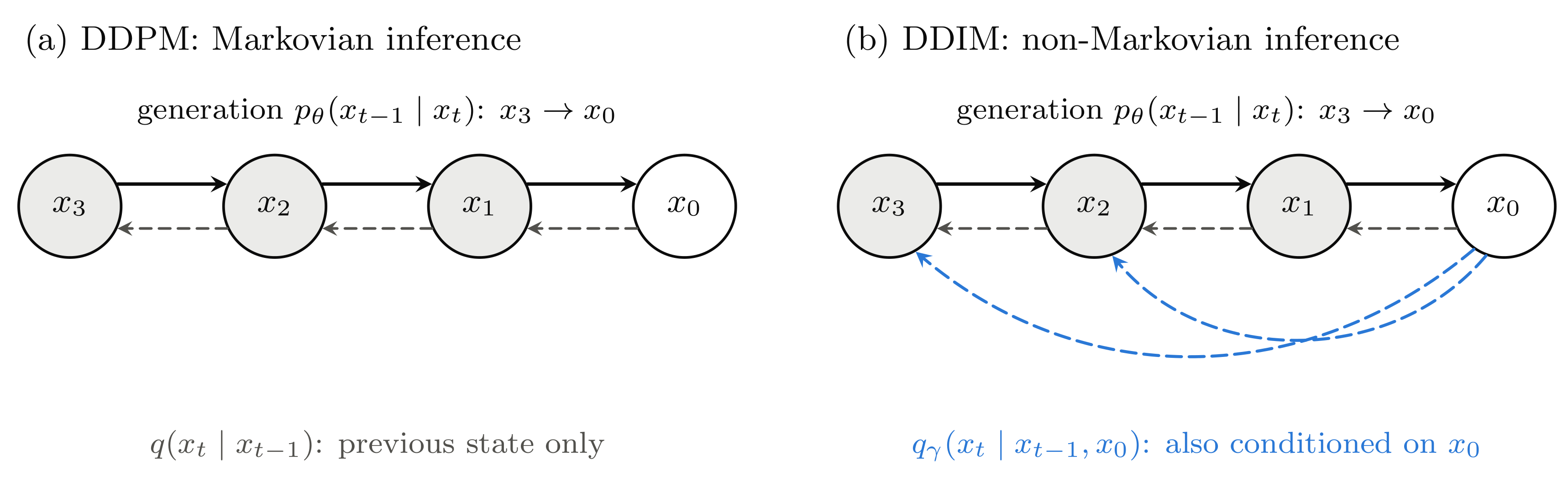
Figure 6.1 summarizes the structure of DDPM. The solid arrows p_\theta(x_{t-1}\mid x_t), pointing right, form the learned generative chain from the standard Gaussian x_T back to the data x_0; the dashed arrow q(x_t\mid x_{t-1}), pointing left, is the fixed forward transition from data to noise (Ho et al. 2020, fig. 2).
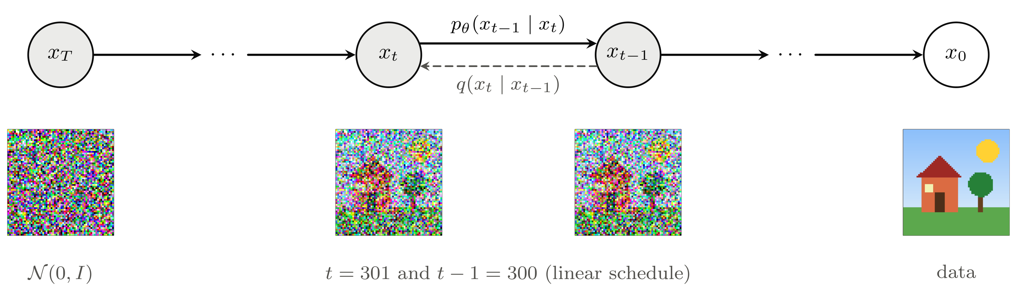
The forward direction repeatedly attenuates the previous state and adds noise until the state is close to a standard Gaussian. The reverse direction models each denoising step as a transition with parameters \mu_\theta and \Sigma_\theta; applying these transitions from x_T to x_0 produces a new sample rather than reconstructing a particular training example. Adding noise is fixed and tractable, whereas reversing the entropy increase requires information stored in the learned parameters. Small forward steps make a Gaussian approximation to each reverse transition plausible.
6.4.1.1 The forward chain
The forward process of DDPM (slide 4) is a Markov chain in the sense of Definition 6.1 with Gaussian transitions (Ho et al. 2020, Eq. 2)
q(x_{1:T}\mid x_0) =\prod_{t=1}^{T}q(x_t\mid x_{t-1}), \qquad q(x_t\mid x_{t-1}) =\mathcal N\!\left(\sqrt{1-\beta_t}\,x_{t-1},\beta_t I\right) =\mathcal N\!\left(\sqrt{\alpha_t}\,x_{t-1},\beta_t I\right). \tag{6.4}
Reparameterizing the same transition gives
x_t=\sqrt{\alpha_t}x_{t-1}+\sqrt{\beta_t}\epsilon_t, \qquad \epsilon_t\sim\mathcal N(0,I). \tag{6.5}
The factor \sqrt{\alpha_t} shrinks the previous signal and \sqrt{\beta_t} adds fresh noise. Because \alpha_t+\beta_t=1, this step preserves unit covariance, as the energy computation below makes precise. The \{\beta_t\}_{t=1}^{T} are not learned but fixed in advance. This finite variance schedule determines both the forward corruption levels and the coefficients used by the reverse model.
6.4.1.2 Jumping to any time in one step
x_t can be sampled directly from x_0 without running the chain t times. Unrolling Equation 6.5 twice, as on slide 5, gives
\begin{aligned} x_t &=\sqrt{\alpha_t}\left( \sqrt{\alpha_{t-1}}x_{t-2} +\sqrt{\beta_{t-1}}\epsilon_{t-1} \right) +\sqrt{\beta_t}\epsilon_t\\ &=\sqrt{\alpha_t\alpha_{t-1}}\,x_{t-2} +\underbrace{\sqrt{\alpha_t\beta_{t-1}}\,\epsilon_{t-1} +\sqrt{\beta_t}\,\epsilon_t}_{\sim\,\mathcal N(0,\,(1-\alpha_t\alpha_{t-1})I)}. \end{aligned}
The sum of two independent Gaussian noises is again Gaussian, with variance \alpha_t\beta_{t-1}+\beta_t=\alpha_t(1-\alpha_{t-1})+(1-\alpha_t)=1-\alpha_t\alpha_{t-1}. Repeating this argument gives the following result.
Proposition 6.2 (Closed form of the forward marginal) For every t=0,1,\ldots,T there is \bar\epsilon_t\sim\mathcal N(0,I), independent of x_0, such that
\begin{aligned} x_t &=\sqrt{\bar\alpha_t}\,x_0 +\sqrt{1-\bar\alpha_t}\,\bar\epsilon_t, \qquad \bar\alpha_t=\prod_{s=1}^{t}\alpha_s,\\ \text{that is,}\quad q(x_t\mid x_0) &=\mathcal N\!\left( \sqrt{\bar\alpha_t}x_0, (1-\bar\alpha_t)I \right). \end{aligned} \tag{6.6}
Proof. By induction on t; at t=0, \bar\alpha_0=1 and the claim is trivial. Suppose that x_{t-1}=\sqrt{\bar\alpha_{t-1}}x_0+\sqrt{1-\bar\alpha_{t-1}}\,\bar\epsilon_{t-1}, where \bar\epsilon_{t-1} depends only on \epsilon_1,\ldots,\epsilon_{t-1}. Substituting into Equation 6.5 and using \alpha_t\bar\alpha_{t-1}=\bar\alpha_t,
x_t=\sqrt{\bar\alpha_t}\,x_0+\Big(\sqrt{\alpha_t(1-\bar\alpha_{t-1})}\,\bar\epsilon_{t-1}+\sqrt{\beta_t}\,\epsilon_t\Big).
The two noises in the parentheses are independent of each other and of x_0, so by Lemma 6.1 the parenthesis is Gaussian with mean 0 and covariance \big[\alpha_t(1-\bar\alpha_{t-1})+\beta_t\big]I=(1-\bar\alpha_t)I, as in the two-step computation above. Writing it as \sqrt{1-\bar\alpha_t}\,\bar\epsilon_t gives \bar\epsilon_t\sim\mathcal N(0,I), independent of x_0. Equivalently, substituting the induction hypothesis into Equation 6.2 evaluates a Gaussian integral with the same result. \square
This sample representation is the one-step renoising formula:
x_t =\sqrt{\bar\alpha_t}x_0 +\sqrt{1-\bar\alpha_t}\epsilon, \qquad \epsilon\sim\mathcal N(0,I). \tag{6.7}
It matters a great deal for training: after drawing any t, x_t is built with one Gaussian draw, without generating the intermediate states x_1,\ldots,x_{t-1}. As t grows and \bar\alpha_t\to0, the data component disappears and q(x_T\mid x_0)\approx\mathcal N(0,I), so generation can start from x_T\sim\mathcal N(0,I). Multiplying the Markov transitions has therefore produced a direct transition from x_0 to any selected time t.
6.4.1.3 Energy, the noise schedule and the SNR
What “keeping the energy” means. Let \Sigma_{t-1} be the covariance of x_{t-1}. Since \epsilon_t is independent of x_{t-1}, the covariance of the sum in Equation 6.5 is the sum of the two covariances; no Gaussian assumption on x_{t-1} is needed. Hence
\Sigma_t=\alpha_t\Sigma_{t-1}+\beta_tI \quad\Longrightarrow\quad \Sigma_t-I=\alpha_t(\Sigma_{t-1}-I) =\bar\alpha_t(\Sigma_0-I).
If the data have unit covariance, the covariance stays I at every step (variance preserving); otherwise \Sigma_t\to I as \bar\alpha_t\to0. The mean is \mathbb E x_t=\sqrt{\bar\alpha_t}\,\mathbb E x_0\to0.
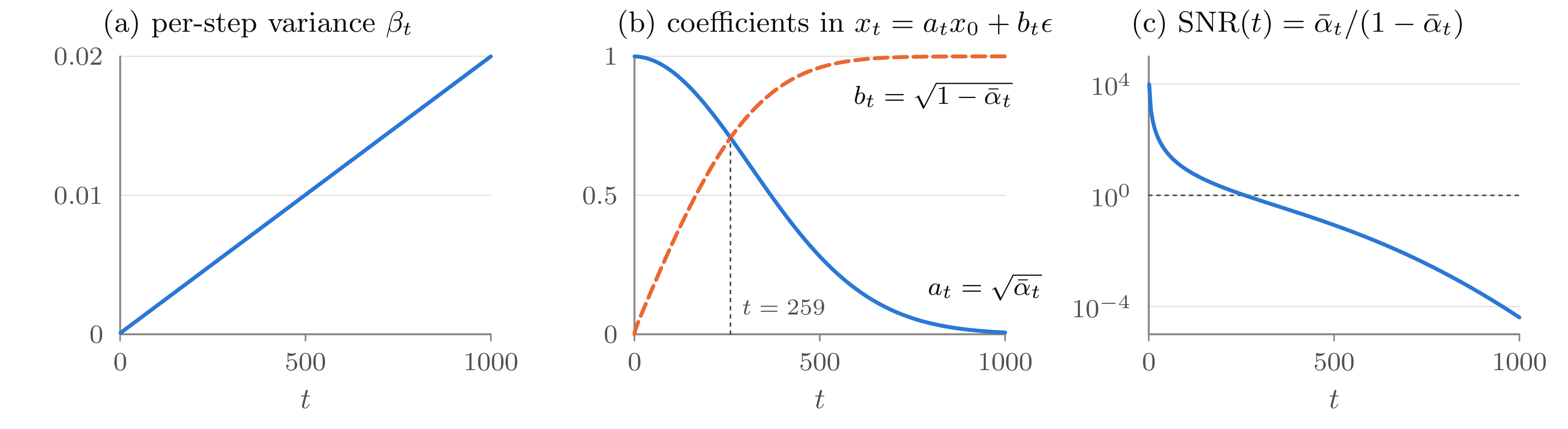
The linear schedule and the signal-to-noise ratio. The size of one step is set by \beta_t, but the signal left at time t is set by \bar\alpha_t, and the corresponding signal-to-noise ratio is \mathrm{SNR}(t)=\bar\alpha_t/(1-\bar\alpha_t). The original paper uses a linear schedule from \beta_1=10^{-4} to \beta_T=0.02 with T=1000 (Ho et al. 2020, sec. 4). As Figure 6.2 shows, \beta_t is linear but \bar\alpha_t decays nonlinearly: signal and noise variances become equal (\bar\alpha_t=\tfrac12) between t=259 and t=260, and \bar\alpha_T\approx4.0\times10^{-5}. The SNR spans more than eight orders of magnitude, from about 10^4 at t=1 to 4\times10^{-5} at t=T, and a uniform t covers them unevenly: the four decades above \mathrm{SNR}=1 get only the first 259 steps, the remaining 4.4 decades the other 741.
curves() in Section 6.6.4.
Other schedules. Nichol and Dhariwal (2021, sec. 3.2) prescribe \bar\alpha_t directly by the cosine schedule \bar\alpha_t=f(t)/f(0), f(t)=\cos^2\!\big(\tfrac{t/T+s}{1+s}\cdot\tfrac{\pi}{2}\big) with s=0.008, and set \beta_t=1-\bar\alpha_t/\bar\alpha_{t-1}, clipped at 0.999. It destroys information more gradually: with T=1000 its \bar\alpha_t is closest to \tfrac12 at t=496, against t=259 for the linear schedule (Section 6.6.4). A schedule is thus best seen as a design of the path of \bar\alpha_t, that is, of the SNR, rather than of \beta_t itself.
6.4.2 The reverse process and the variational bound
6.4.2.1 The generative model
The reverse generative model is
p_\theta(x_{0:T}) =p(x_T)\prod_{t=1}^{T}p_\theta(x_{t-1}\mid x_t), \tag{6.8}
with p(x_T)=\mathcal N(0,I) and, as in Ho et al. (2020), Eq. 1, and on slide 6, each reverse transition modelled as
p_\theta(x_{t-1}\mid x_t) =\mathcal N\!\left( \mu_\theta(x_t,t), \Sigma_\theta(x_t,t) \right).
A common choice fixes \Sigma_\theta(x_t,t)=\sigma_t^2I from the forward schedule and predicts only the mean. The time index is an explicit input because the noise level changes throughout the chain; Ho et al. (2020, sec. 4) feed t to a U-Net through a sinusoidal position embedding. The exact reverse conditional need not be Gaussian. Slide 6 states that in the limit of small steps it has the same functional form as the forward process; the next subsection explains why, and why large jumps require more care.
6.4.2.2 Why the reverse transition is nearly Gaussian for small steps
In Bayes’ rule q(x_{t-1}\mid x_t)\propto q(x_t\mid x_{t-1})\,q_{t-1}(x_{t-1}), the first factor is a narrow Gaussian of width \sqrt{\beta_t/\alpha_t}. Expanding \log q_{t-1} to first order inside that region and applying Lemma 6.2 gives the heuristic approximation (derived in Section 6.9.3)
q(x_{t-1}\mid x_t) \approx \mathcal N\!\left( \frac{x_t}{\sqrt{\alpha_t}}+\frac{\beta_t}{\alpha_t}\nabla\log q_{t-1}\!\Big(\frac{x_t}{\sqrt{\alpha_t}}\Big),\; \frac{\beta_t}{\alpha_t}I \right). \tag{6.9}
One reverse step undoes the forward shrinkage, moves along the score \nabla\log q_{t-1} (the gradient of the log-density) of the marginal, and carries noise of the same size as the forward step. The approximation keeps the slope of \log q_{t-1} across one step and drops its curvature. For sharply concentrated data the dropped term has relative size of the order of
\frac{\beta_t}{\alpha_t(1-\bar\alpha_{t-1})} =\frac{\mathrm{SNR}(t-1)}{\mathrm{SNR}(t)}-1, \tag{6.10}
the relative drop of the SNR over one step. The error has two sources.
- Gaussian data. The exact reverse conditional is Gaussian, but the variance of Equation 6.9 is too large by a relative amount that is at most this ratio, and reaches it as the data variance goes to zero; the mean errs only at second order (Section 6.9.3).
- Non-Gaussian data. The exact reverse conditional is not Gaussian at all. If \log q_{t-1} is smooth, with curvature bounded on the scale \sqrt{\beta_t} of one step, this error comes from the dropped higher-order terms of the expansion and also vanishes as \beta_t\to0.
Both errors are small when the noise variance of one step is much smaller than the noise variance accumulated so far. This is a scale rather than a sharp condition, since between well-separated modes the curvature of \log q_{t-1} can be larger. For the linear schedule the ratio is largest at t=2, about 1.2, and at t=1 it is undefined, so the last step x_1\to x_0 is the hardest to approximate by a Gaussian.
6.4.2.3 An upper bound on the negative log-likelihood
The goal is a small negative log-likelihood. Multiplying and dividing by the forward path distribution, as on slide 7, gives
p_\theta(x_0) =\int p_\theta(x_{0:T})\,dx_{1:T} =\int q(x_{1:T}\mid x_0) \frac{p_\theta(x_{0:T})}{q(x_{1:T}\mid x_0)}\,dx_{1:T} =\mathbb E_{q}\!\left[ \frac{p_\theta(x_{0:T})}{q(x_{1:T}\mid x_0)} \right],
and by Jensen’s inequality
\mathbb E\!\left[-\log p_\theta(x_0)\right] \le \mathbb E_q\!\left[ -\log\frac{p_\theta(x_{0:T})}{q(x_{1:T}\mid x_0)} \right] =:\mathcal L_{\mathrm{VLB}}. \tag{6.11}
Minimizing \mathcal L_{\mathrm{VLB}} therefore minimizes an upper bound on the negative log-likelihood. Substituting p_\theta(x_{0:T})=p_\theta(x_0)\,p_\theta(x_{1:T}\mid x_0) shows that for fixed x_0 the gap of the bound is D_{\mathrm{KL}}\big(q(x_{1:T}\mid x_0)\,\Vert\,p_\theta(x_{1:T}\mid x_0)\big), so the bound is tight only when the forward path distribution equals the model’s posterior over paths.
6.4.2.4 Decomposing the variational bound
Theorem 6.1 (Decomposition of the variational bound) For Equation 6.4 and Equation 6.8,
\begin{aligned} \mathcal L_{\mathrm{VLB}} &=\underbrace{ \mathbb E_q\!\left[ D_{\mathrm{KL}}\!\left(q(x_T\mid x_0)\,\Vert\,p(x_T)\right) \right]}_{L_T}\\ &\quad+ \sum_{t=2}^{T} \underbrace{ \mathbb E_q\!\left[ D_{\mathrm{KL}}\!\left( q(x_{t-1}\mid x_t,x_0) \,\Vert\, p_\theta(x_{t-1}\mid x_t) \right) \right]}_{L_{t-1}}\\ &\quad+ \underbrace{ \mathbb E_q\!\left[-\log p_\theta(x_0\mid x_1)\right] }_{L_0}. \end{aligned} \tag{6.12}
The algebra of slides 7–9 turns Equation 6.11 into Equation 6.12 in three steps; the full proof with every change of measure justified is in Section 6.9.4.
First, substituting Equation 6.4 and Equation 6.8, the loss is
\mathcal L_{\mathrm{VLB}} =\mathbb E_q\!\left[ -\log p(x_T) -\sum_{t\ge1} \log\frac{p_\theta(x_{t-1}\mid x_t)}{q(x_t\mid x_{t-1})} \right]. \tag{6.13}
Next, the Markov property and Bayes’ rule rewrite the denominator for t\ge2:
q(x_t\mid x_{t-1}) =q(x_t\mid x_{t-1},x_0) =q(x_{t-1}\mid x_t,x_0) \frac{q(x_t\mid x_0)}{q(x_{t-1}\mid x_0)}. \tag{6.14}
Setting the t=1 term aside and substituting this identity for t\ge2, the terms \log q(x_{t-1}\mid x_0)-\log q(x_t\mid x_0) telescope (slide 8):
\sum_{t\ge1}\log\frac{p_\theta(x_{t-1}\mid x_t)}{q(x_t\mid x_{t-1})} =\sum_{t=2}^{T}\log\frac{p_\theta(x_{t-1}\mid x_t)}{q(x_{t-1}\mid x_t,x_0)} +\log p_\theta(x_0\mid x_1) -\log q(x_T\mid x_0).
The telescoping sum is why all intermediate marginal-density terms disappear. Substituting it into Equation 6.13 and reading the expectations under q of the log-ratios as KL divergences gives Equation 6.12.
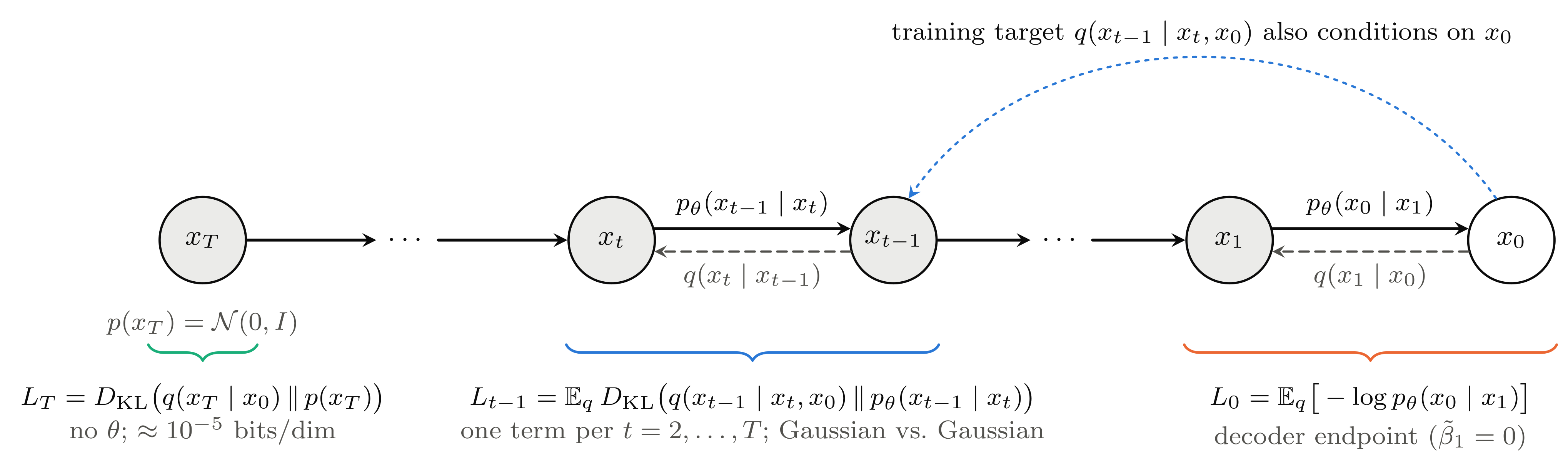
The roles of the terms are as follows. L_T measures how close the last forward distribution is to the prior and does not depend on \theta. L_{t-1} matches one reverse step to the computable exact posterior; it is the main training signal of DDPM. The target q(x_{t-1}\mid x_t,x_0) can be computed during training because x_0 is known. L_0 is the negative log-likelihood of the final reconstruction x_1\to x_0. The Markov factorization and telescoping identity are what reduce a path-space expectation to this sum of local terms.
Figure 6.3 shows where on the chain each kind of term sits.
6.4.2.5 The end terms of the bound
The prior term L_T. L_T has a closed form. Substituting m_1=\sqrt{\bar\alpha_T}x_0, s_1^2=1-\bar\alpha_T, m_2=0, s_2^2=1 into Lemma 6.3,
D_{\mathrm{KL}}\!\left(q(x_T\mid x_0)\,\Vert\,\mathcal N(0,I)\right) =\frac12\left[\bar\alpha_T\left(\lVert x_0\rVert^2-d\right)-d\log(1-\bar\alpha_T)\right] \approx\frac12\bar\alpha_T\lVert x_0\rVert^2.
Since \lVert x_0\rVert^2\le d for data scaled to [-1,1]^d, the bracket is at most -d\log(1-\bar\alpha_T), so L_T\le-\tfrac d2\log(1-\bar\alpha_T). Per dimension, L_T/d\le-\tfrac12\log(1-\bar\alpha_T)\approx2.0\times10^{-5} nats \approx2.9\times10^{-5} bits, and Ho et al. (2020) report about 10^{-5} bits/dim on real data (Sec. 4). The cost of q(x_T\mid x_0)\approx\mathcal N(0,I) is negligible.
The decoder term L_0. Ho et al. (2020) scale the 8-bit pixel values \{0,\ldots,255\} linearly to [-1,1], so neighbouring values are 2/255 apart, and use the discrete decoder (Sec. 3.3, Eq. 13)
\begin{aligned} p_\theta(x_0\mid x_1) &=\prod_{i=1}^{d}\int_{\delta_-(x_0^i)}^{\delta_+(x_0^i)} \mathcal N\!\left(x;\mu_\theta^i(x_1,1),\sigma_1^2\right)dx,\\ \delta_+(x) &= \begin{cases} \infty, & x=1,\\ x+\tfrac{1}{255}, & x<1, \end{cases}\\ \delta_-(x) &= \begin{cases} -\infty, & x=-1,\\ x-\tfrac{1}{255}, & x>-1. \end{cases} \end{aligned} \tag{6.15}
where i indexes the coordinates. Each factor is the probability of the bin of width 2/255 around the observed value, with the two edge bins extended to infinity, so L_0, and with it the whole bound, is a code length for discrete data; Equation 6.11 then bounds a discrete negative log-likelihood by the same Jensen argument. The decoder needs its own positive variance \sigma_1^2, because the choice \sigma_t^2=\tilde\beta_t adopted below gives \tilde\beta_1=0; for concreteness this chapter takes \sigma_1^2=\beta_1. This is a convention of the chapter, not a value stated by Ho et al. (2020); any value of the same order, such as \tilde\beta_2\approx5.5\times10^{-5}, behaves the same way below.
6.4.3 The forward posterior
Computing L_{t-1} requires q(x_{t-1}\mid x_t,x_0). As on slide 10, Bayes’ rule and the Markov property give
\begin{aligned} q(x_{t-1}\mid x_t,x_0) &=\frac{ q(x_t\mid x_{t-1})\,q(x_{t-1}\mid x_0) }{q(x_t\mid x_0)}\\ &=\frac{\mathcal N(x_t;\sqrt{\alpha_t}x_{t-1},\beta_tI)\;\mathcal N(x_{t-1};\sqrt{\bar\alpha_{t-1}}x_0,(1-\bar\alpha_{t-1})I)}{\mathcal N(x_t;\sqrt{\bar\alpha_t}x_0,(1-\bar\alpha_t)I)}. \end{aligned}
The numerator is a product of two Gaussians, the second of which is the one-step marginal Equation 6.6, and the denominator does not depend on x_{t-1}. Expanding the squared norms in the exponents and keeping only the terms that contain x_{t-1},
\log q(x_{t-1}\mid x_t,x_0) =-\frac12\left(\frac{\alpha_t}{\beta_t}+\frac{1}{1-\bar\alpha_{t-1}}\right)\lVert x_{t-1}\rVert^2 +\left(\frac{\sqrt{\alpha_t}}{\beta_t}x_t+\frac{\sqrt{\bar\alpha_{t-1}}}{1-\bar\alpha_{t-1}}x_0\right)^{\!\mathsf T}x_{t-1} +\text{const},
and completing the square (Lemma 6.2) gives the following (slides 10–11).
Proposition 6.3 (Forward posterior) For t\ge2, q(x_{t-1}\mid x_t,x_0)=\mathcal N\!\left(\tilde\mu_t(x_t,x_0),\tilde\beta_tI\right) with
\begin{aligned} \tilde\mu_t(x_t,x_0) &=\frac{ \sqrt{\alpha_t}(1-\bar\alpha_{t-1})}{1-\bar\alpha_t}\,x_t +\frac{\sqrt{\bar\alpha_{t-1}}\,\beta_t}{1-\bar\alpha_t}\,x_0,\\ \tilde\beta_t &=\frac{1-\bar\alpha_{t-1}}{1-\bar\alpha_t}\beta_t. \end{aligned} \tag{6.16}
Proof. By Lemma 6.2 the precision is the coefficient of -\tfrac12\lVert x_{t-1}\rVert^2 above and the variance is its inverse. Putting the precision over a common denominator and using \bar\alpha_t=\alpha_t\bar\alpha_{t-1} and \alpha_t+\beta_t=1,
\frac{\alpha_t}{\beta_t}+\frac{1}{1-\bar\alpha_{t-1}} =\frac{\alpha_t(1-\bar\alpha_{t-1})+\beta_t}{\beta_t(1-\bar\alpha_{t-1})} =\frac{1-\bar\alpha_t}{\beta_t(1-\bar\alpha_{t-1})}=\frac{1}{\tilde\beta_t}.
The mean is the variance \tilde\beta_t times the linear coefficient, and multiplying out, \tilde\beta_t\sqrt{\alpha_t}/\beta_t=\sqrt{\alpha_t}(1-\bar\alpha_{t-1})/(1-\bar\alpha_t) and \tilde\beta_t\sqrt{\bar\alpha_{t-1}}/(1-\bar\alpha_{t-1})=\sqrt{\bar\alpha_{t-1}}\,\beta_t/(1-\bar\alpha_t). \square
It is important that this distribution is conditioned on the clean x_0 as well as on x_t. During training x_0 is known, so the target can be computed; during generation it is not, so p_\theta(x_{t-1}\mid x_t) has to approximate the resulting reverse conditional. DDIM will preserve the same noisy marginals while changing how the latent path depends on x_0.
6.4.3.1 Choice of the reverse variance
Slide 13 fixes the reverse variance to \sigma_t^2:=\tilde\beta_t, one of the two fixed choices of Ho et al. (2020, sec. 3.2); the other is \sigma_t^2=\beta_t. The former is optimal when x_0 is a single point, the latter when x_0\sim\mathcal N(0,I), and the two give similar results. Neither is chosen freely at each step: the forward schedule \{\beta_t\} determines both in closed form. Their ratio \tilde\beta_t/\beta_t=(1-\bar\alpha_{t-1})/(1-\bar\alpha_t) is close to 1 except at small t (Nichol and Dhariwal 2021, sec. 3.1, Fig. 1), the same region where the Gaussian approximation of Section 6.4.2.2 is worst. At t=1, \tilde\beta_1=0 means that the forward posterior is a point mass, not that a logarithm of 0 must be computed; this endpoint is handled by L_0, and the sampler sets z=0 at the last step.
6.4.4 From mean prediction to noise prediction
6.4.4.1 Simplifying the Gaussian KL divergence
With the reverse variance fixed, L_{t-1} is a KL divergence between two Gaussians: one is the posterior computed from the real data, the other the parameterized model to be estimated by a neural network. Choosing different variances leaves an additional variance term; choosing them equal leaves only the squared distance between the means (Lemma 6.3). Hence (slide 12)
L_{t-1} =\mathbb E_q\!\left[ \frac{1}{2\sigma_t^2} \left\lVert \tilde\mu_t(x_t,x_0)-\mu_\theta(x_t,t) \right\rVert^2 \right] +C_t, \tag{6.17}
where C_t\ge0 is a constant independent of \theta that vanishes when \sigma_t^2=\tilde\beta_t (Section 6.9.5).
6.4.4.2 Replacing the dependence on the data by the noise
The target \tilde\mu_t in Equation 6.17 depends on x_0, which the network has to infer from x_t at generation time. As on slide 12, inverting the one-step renoising formula Equation 6.7 rewrites that dependence as one on the noise, so that the network can be asked to predict the noise instead: x_0=(x_t-\sqrt{1-\bar\alpha_t}\,\epsilon)/\sqrt{\bar\alpha_t}. Substituting this expression into Equation 6.16,
\begin{aligned} \tilde\mu_t &=\frac{\sqrt{\alpha_t}(1-\bar\alpha_{t-1})\,x_t+\beta_t\sqrt{\bar\alpha_{t-1}}\,\frac{1}{\sqrt{\bar\alpha_t}}\left(x_t-\sqrt{1-\bar\alpha_t}\,\epsilon\right)}{1-\bar\alpha_t}\\ &=\frac{1}{\sqrt{\alpha_t}}\left(\frac{\alpha_t-\bar\alpha_t+\beta_t}{1-\bar\alpha_t}\,x_t-\frac{\beta_t\sqrt{1-\bar\alpha_t}}{1-\bar\alpha_t}\,\epsilon\right) =\frac{1}{\sqrt{\alpha_t}} \left( x_t- \frac{\beta_t}{\sqrt{1-\bar\alpha_t}}\epsilon \right). \end{aligned} \tag{6.18}
The second line factors out 1/\sqrt{\alpha_t} using \sqrt{\bar\alpha_{t-1}}/\sqrt{\bar\alpha_t}=1/\sqrt{\alpha_t} and \sqrt{\alpha_t}(1-\bar\alpha_{t-1})=(\alpha_t-\bar\alpha_t)/\sqrt{\alpha_t}; the last equality holds because \alpha_t+\beta_t=1 makes the numerator 1-\bar\alpha_t. The exact posterior mean is now expressed through x_t and the noise \epsilon that produced it.
6.4.4.3 The noise parameterization and its loss
\tilde\mu_t is a training target computed from the data, whereas the network estimates \mu_\theta. Following Equation 6.18, the network can be parameterized to predict the noise \epsilon_\theta(x_t,t) instead of the mean (slide 13):
\mu_\theta(x_t,t) :=\frac{1}{\sqrt{\alpha_t}} \left( x_t- \frac{\beta_t}{\sqrt{1-\bar\alpha_t}} \epsilon_\theta(x_t,t) \right). \tag{6.19}
The difference of the two means is a constant multiple of the difference of the noises,
\tilde\mu_t-\mu_\theta =\frac{\beta_t}{\sqrt{\alpha_t}\sqrt{1-\bar\alpha_t}}\left(\epsilon_\theta(x_t,t)-\epsilon\right).
Substituting this relation into Equation 6.17 and replacing the expectation over x_t by one over (x_0,\epsilon) through Equation 6.7 gives the loss of slide 13,
\begin{aligned} L_{t-1} &=w_t\, \mathbb E_{x_0,\epsilon}\!\left[ \left\lVert \epsilon- \epsilon_\theta\!\left( \sqrt{\bar\alpha_t}x_0 +\sqrt{1-\bar\alpha_t}\epsilon, t \right) \right\rVert^2 \right] +C_t,\\ w_t &:=\frac{\beta_t^2} {2\sigma_t^2\alpha_t(1-\bar\alpha_t)}. \end{aligned} \tag{6.20}
This trains the network to estimate the noise used to construct x_t at the selected noise level. The noise-prediction MSE is therefore not an arbitrary surrogate: it is the Gaussian reverse-mean matching objective written in observable training variables.
6.4.4.4 The simplified objective
In practice DDPM drops the time coefficient w_t of Equation 6.20 and trains on the following objective, the loss minimized by Algorithm 1 on slide 14 (Ho et al. 2020, Eq. 14):
\mathcal L_{\mathrm{simple}} =\mathbb E_{\substack{ x_0\sim q_{\mathrm{data}},\\ t\sim\mathrm{Unif}\{1,\ldots,T\},\\ \epsilon\sim\mathcal N(0,I) }} \left[ \left\lVert \epsilon- \epsilon_\theta(x_t,t) \right\rVert^2 \right], \quad x_t=\sqrt{\bar\alpha_t}x_0 +\sqrt{1-\bar\alpha_t}\epsilon. \tag{6.21}
6.4.4.5 The simplified objective is a reweighted ELBO
Dropping w_t changes how training effort is distributed over noise levels. The next calculation makes explicit what changes, what stays fixed at the population optimum, and why the reweighting can improve samples.
What changes. Apart from the end terms L_T and L_0, discussed below, \mathcal L_{\mathrm{VLB}} is \sum_{t\ge2}w_t\,\mathbb E\lVert\epsilon-\epsilon_\theta\rVert^2 plus a constant, and \mathcal L_{\mathrm{simple}} replaces every w_t by 1, up to the factor 1/T from averaging over t (its t=1 term corresponds to L_0, as shown below). For the two fixed variance choices,
\begin{aligned} \sigma_t^2=\tilde\beta_t:&\quad w_t=\frac{\beta_t^2(1-\bar\alpha_t)}{2\alpha_t(1-\bar\alpha_t)(1-\bar\alpha_{t-1})\beta_t} =\frac{\beta_t}{2\alpha_t(1-\bar\alpha_{t-1})},\\ \sigma_t^2=\beta_t:&\quad w_t=\frac{\beta_t}{2\alpha_t(1-\bar\alpha_t)}. \end{aligned} \tag{6.22}
The ratio \beta_t/(\alpha_t(1-\bar\alpha_{t-1})) in the first expression is the ratio Equation 6.10 that set the heuristic error scale of the Gaussian approximation in Section 6.4.2.2. Written with the SNR,
w_t=\frac12\left(\frac{\mathrm{SNR}(t-1)}{\mathrm{SNR}(t)}-1\right) \qquad(\sigma_t^2=\tilde\beta_t), \tag{6.23}
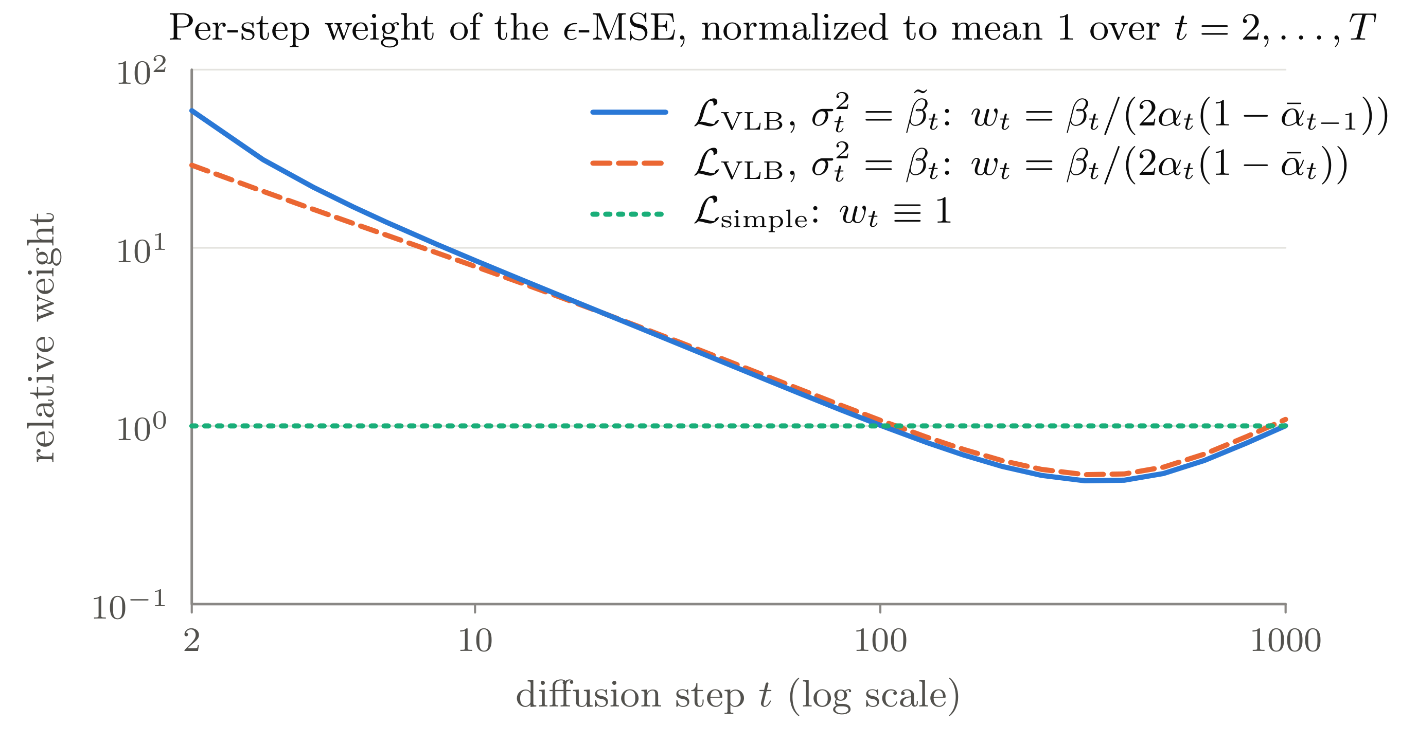
so the exact VLB weights the noise-prediction error at each step by the relative loss of SNR in that step. Table 6.2 quantifies this for the linear schedule. With \sigma_t^2=\tilde\beta_t the weight at t=2 is about 59 times the mean, and for t\le100 it decays roughly like 1/t (Figure 6.4). The first 1% of the chain carries 18.4% of the total weight, against 0.9% under \mathcal L_{\mathrm{simple}}. The exact VLB thus concentrates the training signal on easy denoising problems with almost no noise, and \mathcal L_{\mathrm{simple}} sharply lowers their share.
| \sigma_t^2 / loss | t=2 | t=10 | t=100 | t=500 | share of t\le10 | share of t\le100 |
|---|---|---|---|---|---|---|
| VLB, \tilde\beta_t | 58.9 | 8.49 | 1.01 | 0.54 | 18.4% | 39.2% |
| VLB, \beta_t | 29.1 | 7.87 | 1.08 | 0.59 | 12.8% | 34.1% |
| \mathcal L_{\mathrm{simple}} | 1 | 1 | 1 | 1 | 0.9% | 9.9% |
What does not change. If the network can represent an arbitrary function of x_t for each t, then for any positive weights \{\lambda_t\} the minimizer of \sum_t\lambda_t\mathbb E\lVert\epsilon-\epsilon_\theta(x_t,t)\rVert^2 is the same,
\epsilon^*(x_t,t)=\mathbb E[\epsilon\mid x_t] \tag{6.24}
(Section 6.9.6). The weights matter only in the practical situation where one finite network is shared across all t: they decide how capacity and gradient are allocated across noise levels.
What it buys. Ho et al. (2020) explain that the simplified loss lowers the weight of the small-t terms, the easy tasks of removing very little noise, so that the network can focus on the harder denoising tasks at larger t, and that this improves sample quality (Sec. 3.4). On CIFAR-10, training on the exact VLB with a fixed isotropic variance gave IS 7.67, FID 13.51 and NLL \le 3.70 bits/dim, while \mathcal L_{\mathrm{simple}} gave IS 9.46, FID 3.17 and NLL \le 3.75 bits/dim (Ho et al. 2020, Tables 1–2). The reweighting trades a little log-likelihood for a large gain in sample quality. This benefit is empirical: the numerical examples of this chapter use the Bayes-optimal predictor, for which the weights do not matter (Equation 6.24), so they cannot show it; Nichol and Dhariwal (2021) recover much of the lost likelihood by also learning the variance.
The ablation of Ho et al. (2020, sec. 4.2, Table 2) shows why the noise parameterization matters: predicting \tilde\mu_t works only with the true bound (FID 13.22 with a fixed isotropic variance; its unweighted MSE was unstable), whereas predicting \epsilon is about as good under the bound (FID 13.51) and much better under \mathcal L_{\mathrm{simple}} (FID 3.17).
Learning the variance. The constant C_t of Equation 6.17 is independent of \theta only because the variance is fixed. Nichol and Dhariwal (2021) instead learn a diagonal \Sigma_\theta(x_t,t) with entries \exp\!\big(\nu\log\beta_t+(1-\nu)\log\tilde\beta_t\big), an interpolation in the log domain between the two fixed choices, where the network outputs one \nu per dimension (Sec. 3.1). The variance term C_t of the KL divergence then depends on \theta and trains \nu. They minimize \mathcal L_{\mathrm{hybrid}}=\mathcal L_{\mathrm{simple}}+0.001\,\mathcal L_{\mathrm{VLB}} with a stop-gradient on the mean inside \mathcal L_{\mathrm{VLB}}, so the mean keeps the reweighting of \mathcal L_{\mathrm{simple}} while the bound trains the variance. The rest of this chapter keeps the variance fixed, as on the slides.
Why not optimize the bound directly? Besides sample quality there is an optimization reason. The terms of the bound differ by orders of magnitude (Table 6.2), so with t drawn uniformly its gradient is very noisy. Nichol and Dhariwal (2021) keep the bound but sample t with probability proportional to \sqrt{\mathbb E[L_{t-1}^2]} and divide each term by that probability, which leaves the bound unbiased and makes it far less noisy to optimize (Sec. 3.3).
The end terms. The weights w_t above apply only to the interior KL terms, t\ge2; L_T does not depend on \theta. If each bin integral of Equation 6.15 is approximated by density times bin width, -\log p_\theta(x_0\mid x_1) becomes \lVert x_0-\mu_\theta(x_1,1)\rVert^2/(2\sigma_1^2) plus a constant. At t=1, x_1=\sqrt{\alpha_1}x_0+\sqrt{\beta_1}\epsilon and Equation 6.19 give x_0-\mu_\theta(x_1,1)=\sqrt{\beta_1/\alpha_1}\,(\epsilon_\theta-\epsilon), so
L_0\approx\frac{\beta_1}{2\alpha_1\sigma_1^2}\, \mathbb E\lVert\epsilon-\epsilon_\theta(x_1,1)\rVert^2+\text{const},
formally a noise-prediction MSE with weight 1/(2\alpha_1)\approx\tfrac12 for \sigma_1^2=\beta_1: up to this weight, the t=1 term of \mathcal L_{\mathrm{simple}} (Ho et al. 2020, sec. 3.4). The approximation gives the form of the term rather than its value, since the bin width 2/255\approx0.0078 is not small next to \sigma_1=0.01.
Where the bound spends its nats. Figure 6.5 shows the small-t concentration from two sides: in (a), the two fixed variances \tilde\beta_t and \beta_t differ only in the first steps; in (b), the interior terms L_{t-1}, computed exactly for the one-dimensional example of Section 6.6, fall by six orders of magnitude, as the weights of Table 6.2 predict. Nichol and Dhariwal (2021) report the same pattern for a trained image model (Fig. 2).
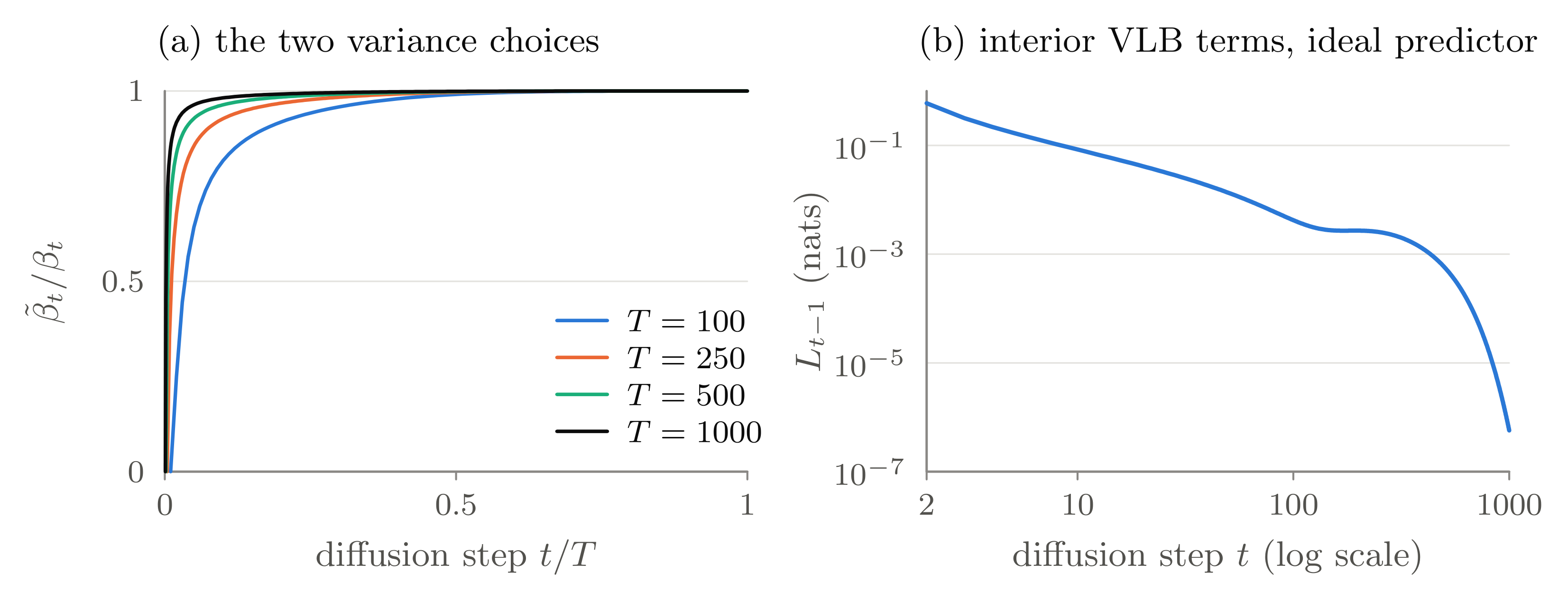
curves() in Section 6.6.4, panel (b) from vlb_terms() in the code of Section 6.6.
6.4.5 Noise, data and velocity prediction
Diffusion models can predict the noise \epsilon, the clean data x_0, or the velocity v. These targets are algebraically interchangeable, but the corresponding MSE objectives weight reconstruction errors differently across noise levels (Salimans and Ho 2022, sec. 4 and App. D).
With a_t=\sqrt{\bar\alpha_t} and b_t=\sqrt{1-\bar\alpha_t} we have x_t=a_tx_0+b_t\epsilon and a_t^2+b_t^2=1.
6.4.5.1 Noise prediction and data prediction
If the network outputs \hat\epsilon=\epsilon_\theta(x_t,t), the data prediction is
\hat x_0 =\frac{x_t-b_t\hat\epsilon}{a_t}, \tag{6.25}
and if it outputs \hat x_0 directly instead,
\hat\epsilon =\frac{x_t-a_t\hat x_0}{b_t}. \tag{6.26}
The two are algebraically equivalent at interior times with a_t,b_t>0. But at very low SNR, a_t\approx0 and the 1/a_t in Equation 6.25 strongly amplifies errors in the noise prediction; at very high SNR, b_t\approx0 and the 1/b_t in Equation 6.26 strongly amplifies errors in the data prediction. Even though they represent the same ideal solution, the conditioning of training differs at finite precision and capacity. For the same reason samplers often clip the data prediction to the data range, \hat x_0\leftarrow\mathrm{clip}(\hat x_0,-1,1), before it is used; this static thresholding keeps samples in range but departs from the exact noise-parameterized mean (Saharia et al. 2022, secs. 2.3, arXiv:2205.11487).
Whichever target is predicted, the DDPM reverse mean is the posterior mean of Equation 6.16 evaluated at the data prediction, \mu_\theta(x_t,t)=\tilde\mu_t(x_t,\hat x_0): substituting Equation 6.25 for x_0 is exactly the computation of Equation 6.18 and gives back Equation 6.19. For the same underlying prediction the three parameterizations therefore define the same sampler; they differ only in what the network is asked to output.
6.4.5.2 Velocity prediction is an orthogonal rotation
Since a_t^2+b_t^2=1, define the angle \phi_t:=\arctan(b_t/a_t)\in(0,\pi/2), so that a_t=\cos\phi_t and b_t=\sin\phi_t. The velocity target is defined as
v:=a_t\epsilon-b_tx_0 =\frac{d x_t}{d\phi_t}\bigg|_{x_0,\epsilon\ \text{fixed}}.
The second equality follows by differentiating x_t=\cos\phi_t\,x_0+\sin\phi_t\,\epsilon with respect to \phi_t, which explains the name “velocity” (Salimans and Ho 2022, App. D). In matrix form,
\begin{bmatrix}x_t\\v\end{bmatrix} = \begin{bmatrix} a_t & b_t\\ -b_t & a_t \end{bmatrix} \begin{bmatrix}x_0\\\epsilon\end{bmatrix},
the two rows are orthogonal and the determinant is a_t^2+b_t^2=1, so the matrix is a rotation: (x_t,v) are the coordinates of the pair (x_0,\epsilon) along axes turned by the angle \phi_t. The inverse is the transpose,
x_0=a_tx_t-b_tv, \qquad \epsilon=b_tx_t+a_tv. \tag{6.27}
For small t, a_t\approx1 and v\approx\epsilon; for large t, b_t\approx1 and v\approx-x_0. A v-predicting network enters the sampler through \hat x_0=a_tx_t-b_t\hat v, that is, through \tilde\mu_t(x_t,\hat x_0) as above.
This is why Salimans and Ho (2022) introduced v-prediction for progressive distillation (Sec. 4). A distilled sampler takes a few large steps and evaluates the network close to \mathrm{SNR}=0, where Equation 6.25 amplifies the error of \hat\epsilon by b_t/a_t\to\infty, whereas \hat x_0=a_tx_t-b_t\hat v from Equation 6.27 stays bounded.
6.4.5.3 Same error, different weights
Converting one prediction into another at the same (x_t,t), Equation 6.25 and Equation 6.27 give \epsilon-\hat\epsilon=\tfrac{a_t}{b_t}(\hat x_0-x_0) and x_0-\hat x_0=-b_t(v-\hat v), hence
\left\lVert\epsilon-\hat\epsilon\right\rVert^2 =\frac{a_t^2}{b_t^2} \left\lVert x_0-\hat x_0\right\rVert^2 =a_t^2\left\lVert v-\hat v\right\rVert^2. \tag{6.28}
Since a_t^2/b_t^2=\mathrm{SNR}(t) and 1/b_t^2=1+\mathrm{SNR}(t),
\lVert\epsilon-\hat\epsilon\rVert^2=\mathrm{SNR}(t)\,\lVert x_0-\hat x_0\rVert^2, \qquad \lVert v-\hat v\rVert^2=\big(1+\mathrm{SNR}(t)\big)\lVert x_0-\hat x_0\rVert^2.
Concretely, Algorithm 1 changes only in its last step. From the same draw (x_0,\epsilon) and the same x_t, x_0-prediction minimizes \lVert x_0-\hat x_0(x_t,t)\rVert^2, and v-prediction computes v=a_t\epsilon-b_tx_0 and minimizes \lVert v-\hat v(x_t,t)\rVert^2; either output is turned into \hat x_0 for the sampler by Equation 6.27. An unweighted \epsilon-MSE is therefore an SNR-weighted error in x_0-space, and an unweighted v-MSE is an “SNR+1”-weighted one (Salimans and Ho 2022, sec. 4). As SNR\to0 (large t), the \epsilon-MSE puts almost no weight on the reconstruction error of x_0, while the v-MSE keeps a weight of at least 1. The three parameterizations are not different generative models but different coordinate systems for the same latent pair; they differ in how much weight the error at each time receives (Figure 6.6).
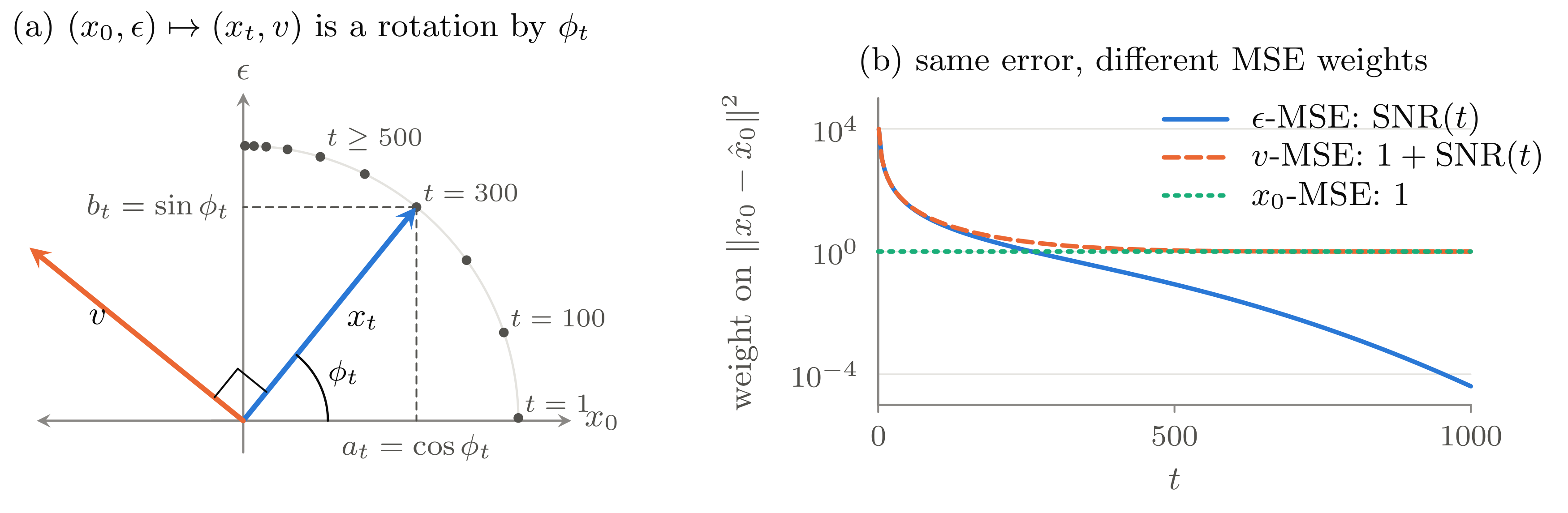
curves() in Section 6.6.4.
Back to the variational bound. The same conversion makes the VLB weights of Equation 6.23 transparent. Multiplying by \mathrm{SNR}(t), which converts an \epsilon-error into an x_0-error by Equation 6.28, each interior term is
L_{t-1} =\frac12\big(\mathrm{SNR}(t-1)-\mathrm{SNR}(t)\big)\, \mathbb E\lVert x_0-\hat x_0(x_t,t)\rVert^2 \qquad(\sigma_t^2=\tilde\beta_t), \tag{6.29}
which is the discrete-time loss of Kingma et al. (2021), Sec. 4, Eq. 13. The VLB weights the x_0-error at a step by the SNR lost in that step, whereas \mathcal L_{\mathrm{simple}} weights it by \mathrm{SNR}(t) itself. In v-space, by the same identities, the VLB weight is \tfrac12\big(\mathrm{SNR}(t-1)-\mathrm{SNR}(t)\big)/\big(1+\mathrm{SNR}(t)\big). The VLB weights sum to \tfrac12\big(\mathrm{SNR}(1)-\mathrm{SNR}(T)\big), and since the linear schedule loses most of its SNR in the first steps (\mathrm{SNR}(1)\approx10^4), most of this total falls on small t.
6.4.6 Training and ancestral sampling
6.4.6.1 The training algorithm
One training iteration of Equation 6.21 is (Ho et al. 2020, Algorithm 1; Ye 2026, slide 14):
- Draw x_0\sim q_{\mathrm{data}}.
- Draw t\sim\mathrm{Unif}\{1,\ldots,T\}.
- Draw the noise \epsilon\sim\mathcal N(0,I), which is therefore known.
- Build x_t in one step with Equation 6.7.
- Update \theta with \nabla_\theta\lVert\epsilon-\epsilon_\theta(x_t,t)\rVert^2.
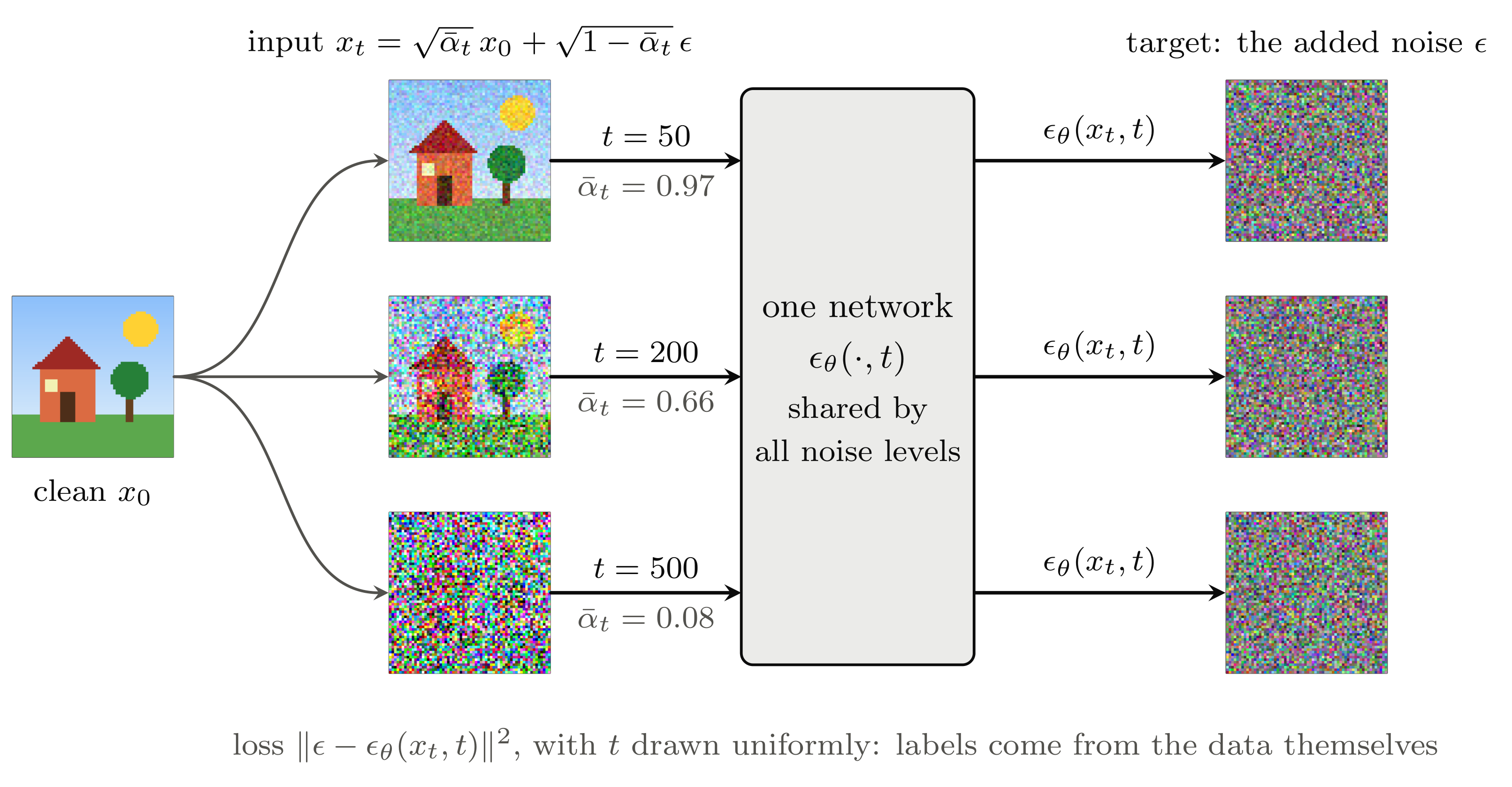
Because the noise is drawn by us and added to clean data, the target \epsilon is known exactly and no human labels are needed. Diffusion training is therefore self-supervised: the model constructs its own input-target pairs. Figure 6.7 shows the same clean image corrupted at several noise strengths, with the network estimating the added noise.
6.4.6.2 Reverse sampling
After training, draw x_T\sim\mathcal N(0,I) and then x_{t-1}\sim p_\theta(x_{t-1}\mid x_t) for each t in turn. This samples the joint p_\theta(x_{0:T}) in ancestral order; apart from the last step, which reports the mean of p_\theta(x_0\mid x_1) instead of a draw from it, the output is a sample of p_\theta(x_0). With Equation 6.19 one step is (slides 13–14)
x_{t-1} =\frac{1}{\sqrt{\alpha_t}} \left( x_t- \frac{\beta_t}{\sqrt{1-\bar\alpha_t}} \epsilon_\theta(x_t,t) \right) +\sigma_t z, \qquad z\sim\mathcal N(0,I). \tag{6.30}
In full (Ho et al. 2020, Algorithm 2):
- Draw x_T\sim\mathcal N(0,I).
- For t=T,T-1,\ldots,1: draw z\sim\mathcal N(0,I) if t>1 and set z=0 if t=1, then compute x_{t-1} with Equation 6.30.
- Return x_0.
The lecture puts the two algorithms side by side and highlights one line in each (Figure 6.8). In training it is the argument of \epsilon_\theta: the noisy image is built in a single jump with Equation 6.7, and no chain is ever simulated. In sampling it is the bracket: the model mean \mu_\theta(x_t,t), to which the fresh noise \sigma_t z is then added. Those two lines are the whole method; everything above derives them.
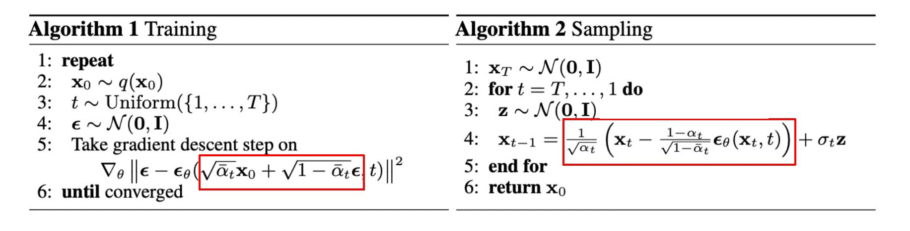
Because 1-\alpha_t=\beta_t, the coefficient in Ho et al. (2020), Algorithm 2 is exactly \beta_t/\sqrt{1-\bar\alpha_t}. The final step sets z=0: the output is \mu_\theta(x_1,1), the mean of the Gaussian inside the decoder, reported without noise (Ho et al. 2020, sec. 3.3). Training costs one network evaluation per sampled time, but ancestral sampling needs T sequential evaluations.
Written out, the two algorithms are shorter than their derivation. Each line below is one of the equations above: x_t is Equation 6.7, loss is Equation 6.21, and the reverse update is Equation 6.30 with \sigma_t^2=\tilde\beta_t.
import torch

def ddpm_training_step(model, x_0, alpha_bar):
    """One training iteration (Algorithm 1)."""
    T = len(alpha_bar) - 1
    t = torch.randint(1, T + 1, (1,)).item()          # t ~ Unif{1,...,T}
    epsilon = torch.randn_like(x_0)                   # the target, known to us
    x_t = (torch.sqrt(alpha_bar[t]) * x_0             # one jump, no chain
           + torch.sqrt(1 - alpha_bar[t]) * epsilon)
    return torch.mean((epsilon - model(x_t, t)) ** 2)

@torch.no_grad()
def ddpm_sample(model, shape, alpha, alpha_bar, sigma):
    """Ancestral sampling (Algorithm 2)."""
    T = len(alpha) - 1
    x_t = torch.randn(shape)                          # x_T ~ N(0, I)
    for t in range(T, 0, -1):
        z = torch.randn_like(x_t) if t > 1 else torch.zeros_like(x_t)
        beta_t = 1 - alpha[t]
        x_t = (1 / torch.sqrt(alpha[t])
               * (x_t - beta_t / torch.sqrt(1 - alpha_bar[t]) * model(x_t, t))
               + sigma[t] * z)
    return x_t
Two details are worth reading off the code. Training never simulates the chain: one draw of t and one of \epsilon give x_t directly, which is why a thousand-step model costs no more per iteration than a ten-step one. Sampling does the opposite, T sequential network evaluations with no way to parallelize over t, and that asymmetry is what the rest of the chapter, and much of the literature after it, works to remove.
Figure 6.9 shows the whole procedure on a two-dimensional example, in the spirit of the first figure of Sohl-Dickstein et al. (2015, sec. 2, Fig. 1). The forward chain spreads the data into noise, ancestral sampling carries the noise back, and the drift field shows how the reverse mean pulls samples towards the data: diffusion moves the whole probability mass, not a single blurred sample.
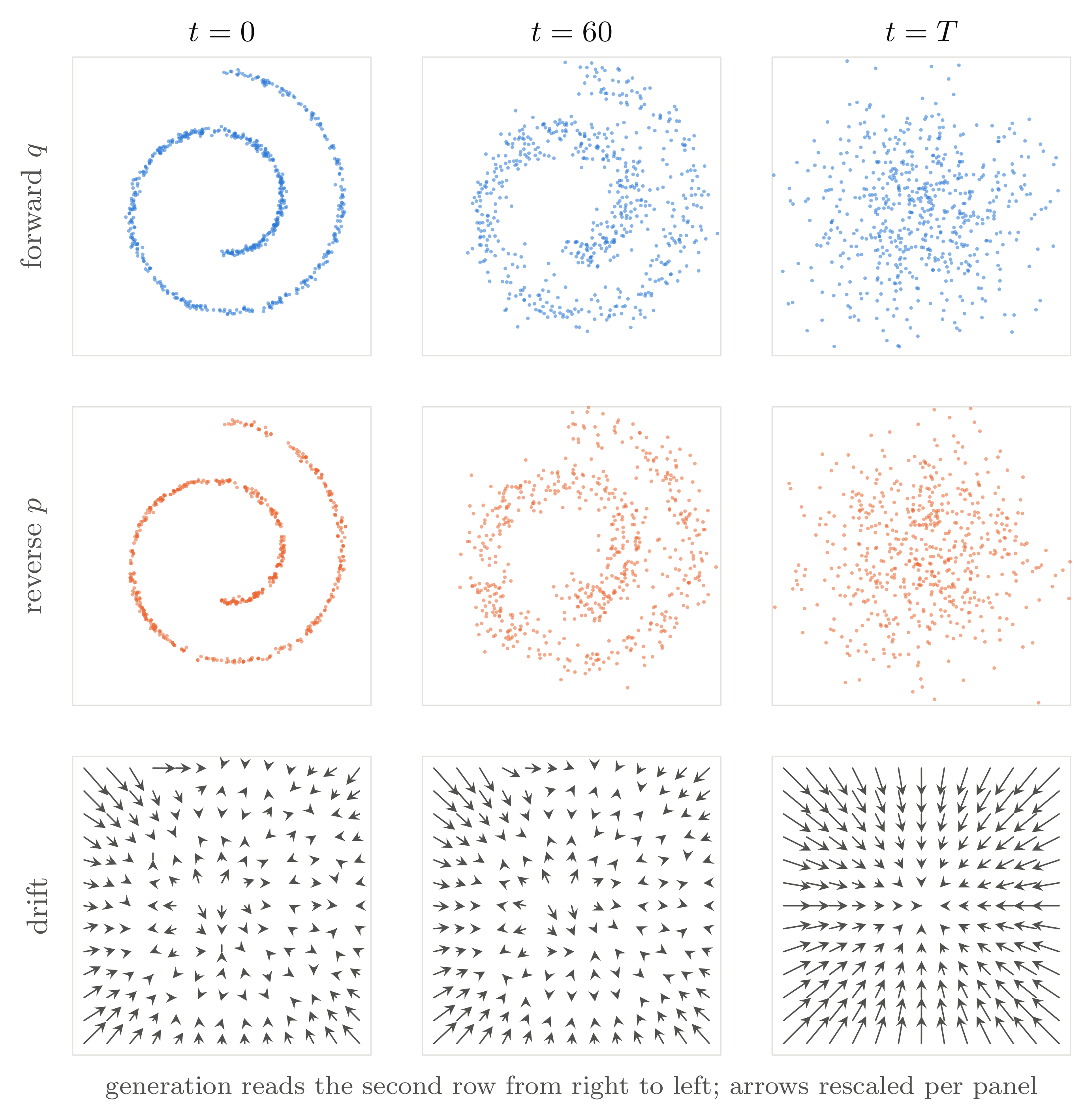
swiss_roll_figure() (Section 6.6.3).
6.4.6.3 Why add noise back to the mean?
Why is \sigma_tz added when \epsilon_\theta has already predicted a noise vector? The two quantities play different roles:
- \epsilon_\theta(x_t,t) is the network output used to compute the conditional mean \mu_\theta(x_t,t);
- z is a fresh random draw used to sample from the conditional Gaussian p_\theta(x_{t-1}\mid x_t) centred at that mean.
DDPM minimizes a KL divergence between the posterior computed from data and a parameterized reverse Gaussian, so both sides are modelled as Gaussian transitions. Sampling from a Gaussian needs the mean plus noise of its standard deviation \sigma_t; using the mean alone picks a single point instead of sampling the conditional distribution. Without the injected noise the reverse chain can contract to almost a single point; the numerical example of Section 6.6 shows this. Removing the noise consistently also changes the mean, which is what DDIM does (Section 6.5).
6.4.6.4 The score, Tweedie’s formula and the DDPM mean
Let q_t(x_t):=\int q_{\mathrm{data}}(x_0)q(x_t\mid x_0)\,dx_0 be the marginal at time t. Under regularity that allows exchanging differentiation and integration (Section 6.9.7),
\nabla\log q_t(x_t) =-\frac{\mathbb E[\epsilon\mid x_t]}{\sqrt{1-\bar\alpha_t}} =-\frac{\epsilon^*(x_t,t)}{\sqrt{1-\bar\alpha_t}}, \qquad \mathbb E[x_0\mid x_t] =\frac{x_t+(1-\bar\alpha_t)\nabla\log q_t(x_t)}{\sqrt{\bar\alpha_t}}. \tag{6.31}
The second identity is Tweedie’s formula; plugging the optimal predictor into \hat x_0 of Equation 6.25 gives exactly this posterior mean. In the same way, writing the DDPM mean Equation 6.19 with the score s_\theta:=-\epsilon_\theta/\sqrt{1-\bar\alpha_t} gives
\mu_\theta(x_t,t)=\frac{1}{\sqrt{\alpha_t}}\Big(x_t+\beta_t\,s_\theta(x_t,t)\Big), \tag{6.32}
which agrees with the mean of the small-step approximation Equation 6.9 to first order in \beta_t. Applying Tweedie’s formula directly to the one-step model x_t=\sqrt{\alpha_t}x_{t-1}+\sqrt{\beta_t}\epsilon_t gives
\mathbb E[x_{t-1}\mid x_t]=\frac{x_t+\beta_t\nabla\log q_t(x_t)}{\sqrt{\alpha_t}} \tag{6.33}
(Section 6.9.7), which is exactly Equation 6.32 with the true score. The ideal DDPM mean is therefore the posterior-mean (Tweedie) denoiser for one step, consistent with the minimizer of Equation 6.17 being \mathbb E[\tilde\mu_t\mid x_t]=\mathbb E[x_{t-1}\mid x_t]. Up to time weights, \epsilon-prediction MSE is therefore denoising score matching (Vincent 2011), the denoising form of the score matching of Hyvarinen (2005).
6.4.6.5 Connection to Noise2Score
Tweedie’s formula (Equation 6.31) connects noise prediction to the score, so one network that estimates the noise, equivalently the score of the noisy data, supplies the information needed for both denoising and generation. Noise2Score (Kim and Ye 2021) learns that score from noisy images alone and applies Tweedie’s formula once and deterministically at the noise level of the image. DDPM sampling applies it iteratively and stochastically over a sequence of noise levels to create a new sample. Training one noise estimator and reusing it, repeatedly and for several downstream tasks such as denoising and generation, is what slide 14 calls the pattern of foundation models: pretraining followed by (iterative) downstream tasks.
6.5 DDIM: a non-Markovian forward process and deterministic sampling
DDIM, the subject of slides 17–25, changes the latent inference path while retaining the same family of noisy marginals (J. Song et al. 2021). Because those marginals determine the denoising inputs, the same noise-prediction network can be reused, under assumptions made precise below. This freedom yields a deterministic sampler and permits generation on a shorter subsequence of times. Slide 17 and the original DDIM paper write DDPM’s \bar\alpha_t as \alpha_t; all equations below use the notation of this chapter (J. Song et al. 2021).
6.5.1 Motivation: is the Markov property needed?
DDPM specifies a Markov forward path and models its small reverse steps with Gaussian transitions. DDIM observes that the simplified loss Equation 6.21 depends on the forward process only through the noisy marginals q(x_t\mid x_0), not through the coupling between different times. It therefore constructs a broader inference family in which a transition can depend directly on the clean endpoint x_0. The blue dashed arrows in Figure 6.10 (b) show this dependence. The generative update (Equation 6.36) still depends on the current state x_t and fresh noise only, so the generative process is Markov; the forward inference distribution q_\gamma is the non-Markovian object.
6.5.2 The non-Markovian forward family
For each sequence \gamma=(\gamma_2,\ldots,\gamma_T) with 0\le\gamma_t^2\le1-\bar\alpha_{t-1}, define the family of slides 19–21 (J. Song et al. 2021, sec. 3.1, Eqs. 6–7)
\begin{aligned} q_\gamma(x_T\mid x_0)&=\mathcal N\!\left(\sqrt{\bar\alpha_T}x_0,(1-\bar\alpha_T)I\right),\\ q_\gamma(x_{1:T}\mid x_0)&=q_\gamma(x_T\mid x_0)\prod_{t=2}^{T}q_\gamma(x_{t-1}\mid x_t,x_0), \end{aligned}
q_\gamma(x_{t-1}\mid x_t,x_0) =\mathcal N\!\left( \sqrt{\bar\alpha_{t-1}}\,x_0 +\sqrt{1-\bar\alpha_{t-1}-\gamma_t^2}\; \frac{x_t-\sqrt{\bar\alpha_t}x_0}{\sqrt{1-\bar\alpha_t}},\; \gamma_t^2I \right). \tag{6.34}
The family is built so that the DDPM marginals survive.
Proposition 6.4 (Marginal preservation) The family Equation 6.34 has the same marginals as DDPM for every t=1,\ldots,T: q_\gamma(x_t\mid x_0)=\mathcal N(\sqrt{\bar\alpha_t}x_0,(1-\bar\alpha_t)I). Slide 20 states the result.
Proof. By backward induction from t=T (J. Song et al. 2021, App. B, Lemma 1). At t=T the claim is the definition. If it holds at t, write x_t=\sqrt{\bar\alpha_t}x_0+\sqrt{1-\bar\alpha_t}\,\epsilon with \epsilon\sim\mathcal N(0,I) and draw x_{t-1} from Equation 6.34 with a fresh z\sim\mathcal N(0,I). Since (x_t-\sqrt{\bar\alpha_t}x_0)/\sqrt{1-\bar\alpha_t}=\epsilon,
x_{t-1}=\sqrt{\bar\alpha_{t-1}}x_0+\sqrt{1-\bar\alpha_{t-1}-\gamma_t^2}\;\epsilon+\gamma_tz,
and since \epsilon and z are independent, Lemma 6.1 gives the mean \sqrt{\bar\alpha_{t-1}}x_0 and the covariance \big[(1-\bar\alpha_{t-1}-\gamma_t^2)+\gamma_t^2\big]I=(1-\bar\alpha_{t-1})I. \square
The coefficient \sqrt{1-\bar\alpha_{t-1}-\gamma_t^2} is essential: with \bar\alpha_t in place of \bar\alpha_{t-1} the covariance would be (1-\bar\alpha_t)I and the induction would break.
With the marginals in hand, the forward-time conditional follows from Bayes’ rule (slide 19):
q_\gamma(x_t\mid x_{t-1},x_0) =q_\gamma(x_{t-1}\mid x_t,x_0)\,\frac{q_\gamma(x_t\mid x_0)}{q_\gamma(x_{t-1}\mid x_0)}.
All three factors are Gaussian, so this conditional can be written out. Given x_0, write x_t=\sqrt{\bar\alpha_t}x_0+\sqrt{1-\bar\alpha_t}\,\epsilon and draw x_{t-1} from Equation 6.34 as x_{t-1}=\sqrt{\bar\alpha_{t-1}}x_0+\sqrt{1-\bar\alpha_{t-1}-\gamma_t^2}\,\epsilon+\gamma_tz. The pair is jointly Gaussian with \mathrm{Cov}(x_t,x_{t-1}\mid x_0)=\sqrt{(1-\bar\alpha_t)(1-\bar\alpha_{t-1}-\gamma_t^2)}\,I and \mathrm{Cov}(x_{t-1}\mid x_0)=(1-\bar\alpha_{t-1})I, and conditioning on x_{t-1} gives, for \gamma_t>0,
q_\gamma(x_t\mid x_{t-1},x_0) =\mathcal N\!\left(\sqrt{\bar\alpha_t}\,x_0+\frac{\sqrt{(1-\bar\alpha_t)(1-\bar\alpha_{t-1}-\gamma_t^2)}}{1-\bar\alpha_{t-1}}\big(x_{t-1}-\sqrt{\bar\alpha_{t-1}}\,x_0\big),\;\frac{(1-\bar\alpha_t)\,\gamma_t^2}{1-\bar\alpha_{t-1}}\,I\right). \tag{6.35}
For \gamma_t^2=\tilde\beta_t the coefficient of x_{t-1} is \sqrt{\alpha_t}, the x_0 terms cancel because \sqrt{\bar\alpha_t}=\sqrt{\alpha_t}\sqrt{\bar\alpha_{t-1}}, and the variance is \beta_t, so Equation 6.35 reduces to the DDPM transition Equation 6.4. For any other \gamma_t this transition depends on the clean image x_0 as well as on the previous state, so the inference path is not Markov, although its marginals are those of DDPM.
Because the marginals are the same, DDIM uses the same one-step renoising inputs as Equation 6.7. The relation between its variational objective and the simplified loss is derived below. The DDIM posterior mean should not be identified with the DDPM mean \tilde\mu_t in general; the two coincide only for the variance choice \gamma_t^2=\tilde\beta_t proved in Proposition 6.5.
6.5.3 The generative step
At generation time x_0 is unknown, so the prediction \hat x_0=(x_t-\sqrt{1-\bar\alpha_t}\,\epsilon_\theta(x_t,t))/\sqrt{\bar\alpha_t} of Equation 6.25 is substituted for x_0 in Equation 6.34 (slides 21–22). Then (x_t-\sqrt{\bar\alpha_t}\hat x_0)/\sqrt{1-\bar\alpha_t}=\epsilon_\theta(x_t,t) exactly, so one step is
x_{t-1} =\underbrace{\sqrt{\bar\alpha_{t-1}}\;\frac{x_t-\sqrt{1-\bar\alpha_t}\,\epsilon_\theta(x_t,t)}{\sqrt{\bar\alpha_t}}}_{\text{predicted }x_0} +\underbrace{\sqrt{1-\bar\alpha_{t-1}-\gamma_t^2}\;\epsilon_\theta(x_t,t)}_{\text{direction pointing to }x_t} +\underbrace{\gamma_t\,z}_{\text{random noise}}. \tag{6.36}
This is the update of slide 17, J. Song et al. (2021), Sec. 4.1, Eq. 12, in the notation of this chapter. Comparing it with Equation 6.30 shows that both the fresh-noise coefficient and the deterministic mean direction depend on \gamma_t.
6.5.4 The exact relation to DDPM and deterministic sampling
Writing both samplers in the same coordinates makes their relation exact.
Proposition 6.5 (Reduction to DDPM) With \gamma_t^2=\tilde\beta_t, Equation 6.34 equals the DDPM posterior \mathcal N(\tilde\mu_t,\tilde\beta_tI). The DDPM ancestral step Equation 6.30 (\sigma_t^2=\tilde\beta_t) can therefore be written
x_{t-1}^{\mathrm{DDPM}} =\sqrt{\bar\alpha_{t-1}}\,\hat x_0+\sqrt{1-\bar\alpha_{t-1}-\tilde\beta_t}\;\epsilon_\theta(x_t,t)+\sqrt{\tilde\beta_t}\,z. \tag{6.37}
Proof in Section 6.9.9.
Deterministic DDIM (\gamma_t=0), on the other hand, is
x_{t-1}^{\mathrm{DDIM}} =\sqrt{\bar\alpha_{t-1}}\,\hat x_0+\sqrt{1-\bar\alpha_{t-1}}\;\epsilon_\theta(x_t,t). \tag{6.38}
The two differ in exactly two places. (i) The variance \tilde\beta_t that DDPM injects as fresh noise is carried deterministically by DDIM along the predicted noise direction \epsilon_\theta, so the coefficient of the “direction pointing to x_t” grows from \sqrt{1-\bar\alpha_{t-1}-\tilde\beta_t} to \sqrt{1-\bar\alpha_{t-1}}. (ii) There is no z term. Seen in the original DDPM form Equation 6.30, this is why the mean looks different and there seems to be an extra \epsilon_\theta term.
Intermediate choices are parameterized as \gamma_t=\eta\sqrt{\tilde\beta_t}, with \eta=1 giving DDPM and \eta=0 giving DDIM (J. Song et al. 2021, sec. 5, Eq. 16). With \gamma_t=0 the whole path down to x_0 is fixed as soon as x_T is fixed, so DDIM is an implicit probabilistic model; the initial x_T is still drawn at random.
6.5.4.1 Denoise, then re-noise
The three terms of Equation 6.36 were named after J. Song et al. (2021), which is how they are usually quoted. The lecture renames them, and the renaming is the point of the slide (slide 23):
x_{t-1} =\underbrace{\sqrt{\bar\alpha_{t-1}}\,\hat x_0(x_t,t)}_{\text{Tweedie's denoiser}} +\underbrace{\sqrt{1-\bar\alpha_{t-1}-\gamma_t^2}\;\epsilon_\theta(x_t,t)}_{\text{parametric noise}} +\underbrace{\gamma_t\,z}_{\text{stochastic noise}} . \tag{6.39}
The first term is not merely a prediction of x_0: by Equation 6.31 it is the Tweedie denoiser of Section 6.4.6.5 applied at noise level t — the same Theorem 5.4 that the previous chapter derived for self-supervised denoising. What the second and third terms do is put the sample back at the noise level t-1, splitting that re-noising between a direction the network computes and a draw that it does not. Every sampler in this chapter is one denoising step followed by one re-noising step, and \eta decides only how much of the re-noising is random.
This also explains why the noise cannot simply be dropped from DDPM while the mean is kept. The marginal of x_{t-1} has to carry variance 1-\bar\alpha_{t-1}; take away the \gamma_t z term and the coefficient of \epsilon_\theta must grow to make up the difference, which is exactly Equation 6.38. The lecture draws this as a sequence of manifolds \mathcal{M}_t, one per noise level, with each step dropping to the data manifold and climbing back to the next one up (slide 24). Keeping that transition on the right manifold is what the later chapters return to.
6.5.5 Why the same network serves every variance choice
The common noise-prediction objective follows from Theorem 1 of J. Song et al. (2021, sec. 3.2). Because q_\gamma(x_{1:T}\mid x_0) is defined directly in reverse order, its variational bound splits into KL terms like Equation 6.12 without the Bayes rearrangement Equation 6.14. In each interior term both Gaussians have covariance \gamma_t^2I, and their means differ only through x_0 versus \hat x_0. Let c_t be the coefficient of x_0 in the mean of Equation 6.34,
c_t:=\sqrt{\bar\alpha_{t-1}}-\sqrt{1-\bar\alpha_{t-1}-\gamma_t^2}\,\sqrt{\frac{\bar\alpha_t}{1-\bar\alpha_t}}>0 .
Then each interior term is a weighted noise-prediction error,
\mathbb E_q\!\left[D_{\mathrm{KL}}\!\left(q_\gamma(x_{t-1}\mid x_t,x_0)\,\Vert\,p_\theta(x_{t-1}\mid x_t)\right)\right] =\lambda_t\,\mathbb E\lVert\epsilon-\epsilon_\theta(x_t,t)\rVert^2, \qquad \lambda_t=\frac{c_t^2}{2\gamma_t^2\,\mathrm{SNR}(t)}, \tag{6.40}
for every \gamma_t>0 (Section 6.9.8). Here p_\theta(x_{t-1}\mid x_t) is the generative step (Equation 6.36), and by Proposition 6.4 the expectation runs over the same pairs x_t=\sqrt{\bar\alpha_t}x_0+\sqrt{1-\bar\alpha_t}\epsilon as \mathcal L_{\mathrm{simple}}. For \gamma_t^2=\tilde\beta_t, \lambda_t reduces to w_t of Equation 6.22, as it must.
Since every \lambda_t is positive, Equation 6.24 applies. If \epsilon_\theta(\cdot,t) can represent any function of x_t for each t, the idealization of Section 6.9.6, then all these objectives and \mathcal L_{\mathrm{simple}} have the same minimizer \mathbb E[\epsilon\mid x_t]. In this sense the network trained for DDPM can be used for any \gamma without retraining. A finite network shared across t only approximates this common minimizer. The deterministic case \gamma_t=0 is not covered by this identity, since \lambda_t\to\infty as \gamma_t\to0. J. Song et al. (2021, sec. 4.1) introduce it as the special case \gamma_t=0 of the generative process and note that, although their Theorem 1 does not cover it, it can be approximated by making \gamma_t very small; every such \gamma shares the minimizer above.
6.5.6 Skipping steps
Choose a subsequence 1=\tau_1<\cdots<\tau_S=T and write Equation 6.34 for each consecutive pair s=\tau_{i-1}<t=\tau_i, with \bar\alpha_s in place of \bar\alpha_{t-1}. The proof of Proposition 6.4 uses only the marginals at the two times involved, so every selected time keeps its marginal; J. Song et al. (2021) attach the unselected times directly to x_0 through q(x_t\mid x_0), which keeps the bound valid and plays no role in sampling [App. C.1]. A model trained with T=1000 can therefore sample in S\ll T steps (J. Song et al. 2021, sec. 4.2). For \eta=1 the variance is the posterior variance of the jump: Proposition 6.3 with \beta_t replaced by the variance 1-\bar\alpha_t/\bar\alpha_s of the forward transition from s to t, and \bar\alpha_{t-1} by \bar\alpha_s. The marginals remain exact for large jumps, but errors in \hat x_0 and discretization errors grow with the jump (Section 6.6). Deterministic sampling tolerates large jumps best: with 20 to 100 steps DDIM gives samples comparable to 1000-step models, a 10 to 50 times speed-up (J. Song et al. 2021, sec. 5.1). In full, generalized DDIM sampling on a subsequence is:
- Choose 1=\tau_1<\cdots<\tau_S=T and \eta\in[0,1], and draw x_{\tau_S}\sim\mathcal N(0,I).
- For i=S,\ldots,1, with t=\tau_i, s=\tau_{i-1} and \tau_0:=0: compute \hat\epsilon=\epsilon_\theta(x_t,t) and \hat x_0 by Equation 6.25, set \gamma^2=\eta^2\frac{1-\bar\alpha_s}{1-\bar\alpha_t}\big(1-\frac{\bar\alpha_t}{\bar\alpha_s}\big), and update x_s=\sqrt{\bar\alpha_s}\,\hat x_0+\sqrt{1-\bar\alpha_s-\gamma^2}\,\hat\epsilon+\gamma z with a fresh z\sim\mathcal N(0,I).
- Return x_0. At the last step \bar\alpha_0=1 gives \gamma=0 and x_0=\hat x_0, the counterpart of reporting the decoder mean in DDPM.
The function ddim in Section 6.6 implements exactly these steps.
6.5.7 DDPM and DDIM side by side
Table 6.3 collects the differences between the two samplers.
| DDPM | DDIM | |
|---|---|---|
| Forward structure | Markov chain linking adjacent states only | non-Markovian family q_\gamma that may depend on x_0 |
| Marginal at each time | Equation 6.6 | same as DDPM (Proposition 6.4) |
| Training | \epsilon_\theta(x_t,t) trained with Equation 6.21 | the same \epsilon_\theta(x_t,t) reused |
| One step | Equation 6.30 | Equation 6.36; with \gamma_t=0, Equation 6.38 |
| Stochasticity | fresh noise at every step | controlled by \eta\in[0,1]; deterministic for \eta=0 |
| Number of steps | all T training steps in Ho et al. (2020); on a subsequence it is DDIM with \eta=1 | any subsequence of S\le T steps |
6.6 Reproducible numerical examples
The following computations check the equations numerically and isolate the difference between the DDPM and DDIM samplers using the Bayes-optimal noise predictor. All code uses only the Python standard library, except the Swiss-roll snippet of Section 6.6.3, which uses NumPy. The plotted figures are drawn with TikZ directly from the values these functions return; the drawing code only places those values on axes.
6.6.1 A two-step scalar example
Fix two steps with x_0=2, (\beta_1,\beta_2)=(0.1,0.2) and (\epsilon_1,\epsilon_2)=(0.5,-1). Then (\alpha_1,\alpha_2,\bar\alpha_2)=(0.9,0.8,0.72), and the forward samples are
\begin{aligned} x_1&=\sqrt{0.9}(2)+\sqrt{0.1}(0.5)\approx2.0555,\\ x_2&=\sqrt{0.8}(2.0555)+\sqrt{0.2}(-1)\approx1.3913,\\ \epsilon &=\frac{x_2-\sqrt{0.72}x_0}{\sqrt{0.28}} \approx-0.5779. \end{aligned}
The variance of the two-step noise is \alpha_2\beta_1+\beta_2=0.28=1-\bar\alpha_2, so the last line is the noise that expresses the same x_2 in one step through Equation 6.7. Substituting the same numbers into Equation 6.16,
\begin{aligned} \tilde\beta_2 &=\frac{1-0.9}{1-0.72}(0.2) =\frac1{14}\approx0.07143,\\ \tilde\mu_2(x_2,x_0) &=\frac{\sqrt{0.8}(1-0.9)(1.3913)+0.2\sqrt{0.9}(2)}{1-0.72} \approx1.7997. \end{aligned}
The actual x_1=2.0555 on this path lies about 0.96 standard deviations above the posterior mean: the posterior mean is the centre of the conditional distribution, not the latent that happened to be drawn.
Assume an oracle predictor that returns exactly the noise of this path, \epsilon_\theta(x_2,2)=\epsilon=-0.5779. Then Equation 6.25 returns \hat x_0=2 exactly, and three updates can be compared:
- Equation 6.18 (the DDPM mean): \frac{1}{\sqrt{0.8}}\big(1.3913-\frac{0.2}{\sqrt{0.28}}(-0.5779)\big)\approx1.7997, equal to \tilde\mu_2.
- Equation 6.36 with \gamma_2^2=\tilde\beta_2: \sqrt{0.9}(2)+\sqrt{0.1-0.07143}(-0.5779)\approx1.7997, equal to the DDPM mean as Proposition 6.5 says.
- Deterministic DDIM (\gamma_2=0): \sqrt{0.9}(2)+\sqrt{0.1}(-0.5779)\approx1.7146. Instead of adding fresh noise, it moves further along the \epsilon direction.
import math
sq = math.sqrt
x0, b1, b2, e1, e2 = 2.0, 0.1, 0.2, 0.5, -1.0
a1, a2 = 1 - b1, 1 - b2
ab1, ab2 = a1, a1 * a2
x1 = sq(a1) * x0 + sq(b1) * e1                    # forward step 1
x2 = sq(a2) * x1 + sq(b2) * e2                    # forward step 2
eps = (x2 - sq(ab2) * x0) / sq(1 - ab2)           # one-step noise
bt = (1 - ab1) / (1 - ab2) * b2                   # beta_tilde_2
mu = (sq(a2) * (1 - ab1) * x2 + b2 * sq(ab1) * x0) / (1 - ab2)
mu_eps = (x2 - b2 / sq(1 - ab2) * eps) / sq(a2)   # epsilon form
x0_hat = (x2 - sq(1 - ab2) * eps) / sq(ab2)       # exact eps given
ddim0 = sq(ab1) * x0_hat + sq(1 - ab1) * eps      # gamma = 0
ddimb = sq(ab1) * x0_hat + sq(1 - ab1 - bt) * eps  # gamma^2 = bt
z = (x1 - mu) / sq(bt)
print(f"x1={x1:.4f} x2={x2:.4f} eps={eps:.4f} beta_tilde={bt:.5f}")
print(f"mu={mu:.4f} mu_eps={mu_eps:.4f} z={z:.3f}")
print(f"x0_hat={x0_hat:.4f} ddim0={ddim0:.4f} ddim_bt={ddimb:.4f}")
# x1=2.0555 x2=1.3913 eps=-0.5779 beta_tilde=0.07143
# mu=1.7997 mu_eps=1.7997 z=0.957
# x0_hat=2.0000 ddim0=1.7146 ddim_bt=1.7997
6.6.2 DDPM and DDIM on a one-dimensional mixture
Using the Bayes-optimal noise predictor \epsilon^*(x_t,t)=\mathbb E[\epsilon\mid x_t] (Equation 6.24), computed analytically, instead of a trained network isolates the properties of the samplers from training error. Note that this is the conditional mean of the noise, not the noise actually added on a path. Take the data to be the one-dimensional Gaussian mixture x_0\sim0.3\,\mathcal N(-1.5,0.2^2)+0.7\,\mathcal N(1,0.3^2). Blurring each component with Equation 6.6 gives q_t(x)=\sum_k\pi_k\mathcal N(x;\sqrt{\bar\alpha_t}\mu_k,V_{t,k}) with V_{t,k}=\bar\alpha_ts_k^2+1-\bar\alpha_t. With the responsibilities r_k(x)=\pi_k\mathcal N(x;\sqrt{\bar\alpha_t}\mu_k,V_{t,k})/q_t(x), Equation 6.31 gives
\epsilon^*(x,t)=-\sqrt{1-\bar\alpha_t}\,\nabla\log q_t(x)=\sqrt{1-\bar\alpha_t}\sum_kr_k(x)\frac{x-\sqrt{\bar\alpha_t}\mu_k}{V_{t,k}}.
With the linear schedule (T=1000), N=4000 draws x_T\sim\mathcal N(0,I) were run through 1000-step DDPM (\sigma_t^2=\tilde\beta_t) and through deterministic DDIM on an evenly spaced subsequence of S steps. Table 6.4 reports the fraction P in the right mode and the mean / standard deviation of each mode (boundary x=-0.25).
| Sampler | Steps S | P(\text{right}) | Left mode | Right mode |
|---|---|---|---|---|
| Target | — | 0.700 | -1.500 / 0.200 | +1.000 / 0.300 |
| DDPM | 1000 | 0.706 | -1.487 / 0.200 | +1.003 / 0.293 |
| DDIM, \eta=0 | 50 | 0.701 | -1.479 / 0.191 | +0.991 / 0.286 |
| DDIM, \eta=0 | 10 | 0.721 | -1.404 / 0.230 | +0.932 / 0.263 |
With N=4000 the standard error of P is about 0.007. Three observations follow.
- Both samplers closely approximate the same target. With \epsilon^*, 1000-step DDPM and 50-step deterministic DDIM (\eta=0) reproduce the target mode fraction to within one standard error, and the mode means and standard deviations to within 0.021 (Figure 6.11 (c)). The remaining discrepancies come from the Gaussian reverse-transition approximation in finite-step DDPM, the discretization error of finite-step DDIM, the small mismatch between q_T and \mathcal N(0,I), and Monte Carlo error. The experiment therefore supports reuse of the same ideal noise predictor without claiming that either finite-step sampler is exact.
- DDIM is deterministic. Started twice from the same x_T=0.3, DDIM returns 0.9608 both times, while DDPM returns different values each time, here -1.4437 and 1.3192, in different modes. In Figure 6.11 (a)–(b), DDPM paths jitter at every step and can reach different modes from the same start, while DDIM paths are smooth and, for these 50 steps, keep the order of their starting points.
- Too few steps fail. At S=10 deterministic DDIM errs clearly: the right-mode fraction is 0.721 against 0.700, the left-mode mean -1.404 against -1.500, and the left-mode spread 0.230 against 0.200. The inference family keeps exact marginals on any subsequence (Section 6.5.6), but the generative chain substitutes \hat x_0 for x_0, and the resulting error grows with the size of each jump.
Dropping the noise of DDPM. Running the DDPM mean with z=0 at every step, from the first 400 of the same draws x_T, sends every sample to x_0\in[0.955,0.965]: without the injected noise the chain here contracts to almost a single point near the larger mode, which is why the sampler of Section 6.4.6 adds \sigma_tz.
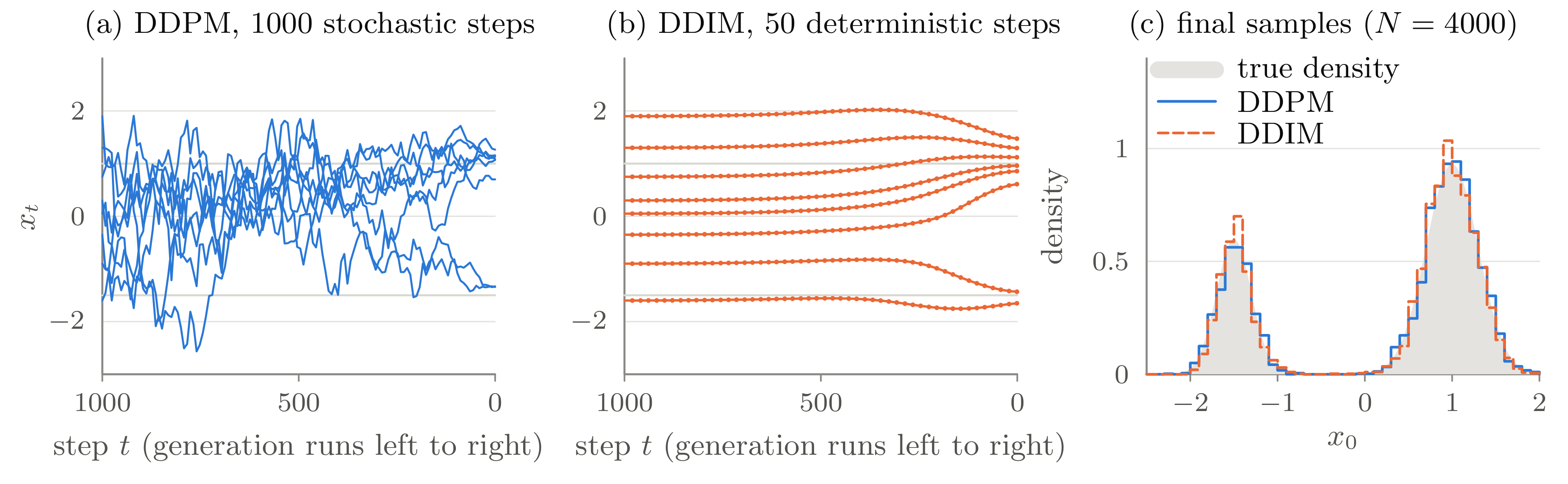
figure_data() in the code below.
The following code reproduces Table 6.4, the determinism check, the z=0 experiment and panel (b) of Figure 6.5 exactly (about 20 seconds with CPython 3.12); its output is listed in the final comments, and figure_data() returns the paths and histograms of Figure 6.11.
import math, random

T = 1000
# beta[t-1] = beta_t, linear from 1e-4 to 0.02
beta = [1e-4 + (0.02 - 1e-4) * i / (T - 1) for i in range(T)]
abar = [1.0]                                  # abar[t], abar[0] = 1
for b in beta:
    abar.append(abar[-1] * (1 - b))

# data: 0.3 N(-1.5, 0.2^2) + 0.7 N(1, 0.3^2)
PI, MU, SD = (0.3, 0.7), (-1.5, 1.0), (0.2, 0.3)

def eps_star(x, t):
    """Exact E[eps | x_t = x] = -sqrt(1 - abar_t) * score."""
    a, logw, z = abar[t], [], []
    for p, m, s in zip(PI, MU, SD):
        var = a * s * s + 1 - a           # Var(x_t | component)
        d = x - math.sqrt(a) * m
        lp = math.log(p) - 0.5 * math.log(var) - d * d / (2 * var)
        logw.append(lp)
        z.append(d / var)
    w = [math.exp(l - max(logw)) for l in logw]
    num = sum(wi * zi for wi, zi in zip(w, z))
    return math.sqrt(1 - a) * num / sum(w)

def ddpm(x, rng, path=None):
    """Ancestral sampling with sigma_t^2 = beta_tilde_t."""
    for t in range(T, 0, -1):
        b = beta[t - 1]
        e = eps_star(x, t)
        mean = (x - b / math.sqrt(1 - abar[t]) * e)
        mean /= math.sqrt(1 - b)
        var = (1 - abar[t - 1]) / (1 - abar[t]) * b
        if t > 1:                             # z = 0 at t = 1
            mean += math.sqrt(var) * rng.gauss(0, 1)
        x = mean
        if path is not None: path.append((t - 1, x))
    return x

def ddim(x, steps=50, eta=0.0, rng=None, path=None):
    """Generalized DDIM on an evenly spaced sub-sequence of 1..T."""
    taus = [round(1 + i * (T - 1) / (steps - 1))
            for i in range(steps)]
    for i in range(steps - 1, -1, -1):
        t, s = taus[i], (taus[i - 1] if i > 0 else 0)
        e = eps_star(x, t)
        x0_hat = (x - math.sqrt(1 - abar[t]) * e)
        x0_hat /= math.sqrt(abar[t])
        r = 1 - abar[t] / abar[s]
        g2 = eta ** 2 * (1 - abar[s]) / (1 - abar[t]) * r
        k = math.sqrt(1 - abar[s] - g2)
        x = math.sqrt(abar[s]) * x0_hat + k * e
        if g2 > 0: x += math.sqrt(g2) * rng.gauss(0, 1)
        if path is not None: path.append((s, x))
    return x

def summary(xs):
    def ms(xs):
        m = sum(xs) / len(xs)
        return m, math.sqrt(sum((u - m) ** 2 for u in xs) / len(xs))
    L = [u for u in xs if u <= -0.25]
    R = [u for u in xs if u > -0.25]
    return len(R) / len(xs), ms(L), ms(R)

def report(name, xs):
    p, (mL, sL), (mR, sR) = summary(xs)
    print(f"{name:13s} P={p:.3f}  L {mL:+.3f}/{sL:.3f}"
          f"  R {mR:+.3f}/{sR:.3f}")

def figure_data():
    """Paths and histograms drawn in the figure."""
    starts = [-1.6, -0.9, -0.35, 0.05, 0.3, 0.75, 1.3, 1.9]
    prng, paths_ddpm, paths_ddim = random.Random(7), [], []
    for x in starts:
        p = [(T, x)]
        ddpm(x, prng, p)
        paths_ddpm.append(p[::8] + [p[-1]])  # every 8th step
        q = [(T, x)]
        ddim(x, 50, path=q)
        paths_ddim.append(q)
    rng = random.Random(0)
    xT = [rng.gauss(0, 1) for _ in range(4000)]
    s_ddpm = [ddpm(x, rng) for x in xT]   # same draws as the table
    s_ddim = [ddim(x, 50) for x in xT]
    lo, hi, nb = -2.5, 2.0, 45
    def hist(xs):                          # density per bin
        cnt = [0] * nb
        for x in xs:
            i = int((x - lo) / (hi - lo) * nb)
            if 0 <= i < nb: cnt[i] += 1
        return [n / (len(xs) * (hi - lo) / nb) for n in cnt]
    return paths_ddpm, paths_ddim, hist(s_ddpm), hist(s_ddim)

def vlb_terms(n=1401):
    """Interior VLB terms L_{t-1} (nats), t = 2..T, with eps*."""
    h, out = 14 / (n - 1), []
    for t in range(2, T + 1):
        a, e2 = abar[t], 0.0
        for i in range(n):
            x = -7 + i * h
            q = sum(p * math.exp(-(x - math.sqrt(a) * m) ** 2
                                 / (2 * (a * s * s + 1 - a)))
                    / math.sqrt(2 * math.pi * (a * s * s + 1 - a))
                    for p, m, s in zip(PI, MU, SD))
            e2 += q * eps_star(x, t) ** 2 * h
        b = beta[t - 1]
        out.append(b / (2 * (1 - b) * (1 - abar[t - 1])) * (1 - e2))
    return out

def ddpm_mean_only(x):
    """DDPM with the noise term dropped: z = 0 at every step."""
    for t in range(T, 0, -1):
        b = beta[t - 1]
        e = eps_star(x, t)
        x = (x - b / math.sqrt(1 - abar[t]) * e) / math.sqrt(1 - b)
    return x

if __name__ == "__main__":
    rng, N = random.Random(0), 4000
    xT = [rng.gauss(0, 1) for _ in range(N)]
    print("target        P=0.700  L -1.500/0.200  R +1.000/0.300")
    report("DDPM, T=1000", [ddpm(x, rng) for x in xT])
    for steps in (50, 10):
        report(f"DDIM, S={steps}", [ddim(x, steps) for x in xT])
    d1, d2 = ddim(0.3), ddim(0.3)
    p1, p2 = ddpm(0.3, rng), ddpm(0.3, rng)
    print("x_T = 0.3: DDIM", round(d1, 4), round(d2, 4),
          "| DDPM", round(p1, 4), round(p2, 4))
    zs = [ddpm_mean_only(x) for x in xT[:400]]
    print("z = 0 throughout: x_0 in [%.3f, %.3f]"
          % (min(zs), max(zs)))
    L = vlb_terms()
    print("VLB terms: L_1 %.2f, L_999 %.1e" % (L[0], L[998]),
          "| share of t<=10: %.1f%%" % (100 * sum(L[:9]) / sum(L)))
# target        P=0.700  L -1.500/0.200  R +1.000/0.300
# DDPM, T=1000  P=0.706  L -1.487/0.200  R +1.003/0.293
# DDIM, S=50    P=0.701  L -1.479/0.191  R +0.991/0.286
# DDIM, S=10    P=0.721  L -1.404/0.230  R +0.932/0.263
# x_T = 0.3: DDIM 0.9608 0.9608 | DDPM -1.4437 1.3192
# z = 0 throughout: x_0 in [0.955, 0.965]
# VLB terms: L_1 0.60, L_999 5.7e-07 | share of t<=10: 42.6%
6.6.3 The Swiss roll
Figure 6.9 uses the exact score of an empirical distribution: with data points d_1,\ldots,d_n, the noisy marginal q_t is a mixture of Gaussians centred at \sqrt{\bar\alpha_t}d_i, and \epsilon^* follows from Equation 6.31 as a softmax-weighted average. The following NumPy code returns the plotted points and arrows (about 40 seconds). Its check, listed in the final comment, confirms the caption: the median distance from a generated sample at t=0 to the nearest training point is 0.0045, far below the 0.03 jitter of the data.
import math
import numpy as np

T = 1000
beta = np.linspace(1e-4, 0.02, T)
abar = np.concatenate([[1.0], np.cumprod(1 - beta)])

def roll(n, rng):
    th = 1.5 * np.pi + 3 * np.pi * rng.random(n)
    p = np.stack([th * np.cos(th), th * np.sin(th)], 1) / 6
    return p + 0.03 * rng.standard_normal(p.shape)

data = roll(1500, np.random.default_rng(0))   # empirical law

def eps_star(x, t):
    """E[eps | x_t = x] under the empirical data law."""
    a, b2 = math.sqrt(abar[t]), 1 - abar[t]
    d2 = ((x[:, None] - a * data[None]) ** 2).sum(-1)
    w = np.exp(-(d2 - d2.min(1, keepdims=True)) / (2 * b2))
    w /= w.sum(1, keepdims=True)
    return (x - a * w @ data) / math.sqrt(b2)

def mean(x, t):                                # DDPM reverse mean
    e = eps_star(x, t)
    return (x - beta[t - 1] / math.sqrt(1 - abar[t]) * e) \
        / math.sqrt(1 - beta[t - 1])

def swiss_roll_figure(times=(0, 60, T)):
    """Forward samples, reverse samples and drift field."""
    x0 = roll(600, np.random.default_rng(1))
    z = np.random.default_rng(2).standard_normal(x0.shape)
    fwd = {t: math.sqrt(abar[t]) * x0 + math.sqrt(1 - abar[t]) * z
           for t in times}
    g = np.random.default_rng(3)
    x = g.standard_normal((600, 2))
    rev = {T: x.copy()}
    for t in range(T, 0, -1):
        var = (1 - abar[t - 1]) / (1 - abar[t]) * beta[t - 1]
        x = mean(x, t)
        if t > 1:
            x = x + math.sqrt(var) * g.standard_normal(x.shape)
        if t - 1 in times:
            rev[t - 1] = x.copy()
    s = np.linspace(-2.4, 2.4, 13)
    grid = np.stack(np.meshgrid(s, s), -1).reshape(-1, 2)
    drift = {t: mean(grid, max(t, 1)) - grid for t in times}
    return fwd, rev, drift

if __name__ == "__main__":
    fwd, rev, drift = swiss_roll_figure()
    d = np.sqrt(((rev[0][:, None] - data[None]) ** 2).sum(-1))
    print("t=0 samples: median distance to nearest data point",
          round(float(np.median(d.min(1))), 4))
# t=0 samples: median distance to nearest data point 0.0045
6.6.4 Schedule and weight statistics
The schedule and weight values quoted in Section 6.4.1.3 (including the cosine schedule), Section 6.4.2.2, Section 6.4.2.5 and Table 6.2 are reproduced by the following code, whose output is listed in the final comments; curves() returns the curves plotted in Figure 6.2, Figure 6.6 (b) and Figure 6.5 (a).
import math

T = 1000
beta = [1e-4 + (0.02 - 1e-4) * i / (T - 1) for i in range(T)]
abar = [1.0]
for b in beta:
    abar.append(abar[-1] * (1 - b))

def snr(t):
    return abar[t] / (1 - abar[t])

def ratio(t):           # beta_t / (alpha_t (1 - abar_{t-1}))
    return beta[t - 1] / ((1 - beta[t - 1]) * (1 - abar[t - 1]))

def curves(TT=1000):
    """beta_t, abar_t, SNR(t) and tilde-beta_t / beta_t of the
    linear schedule shortened to TT steps (ends times 1000/TT)."""
    sc = 1000 / TT
    b = [sc * (1e-4 + (0.02 - 1e-4) * i / (TT - 1))
         for i in range(TT)]
    ab = [1.0]
    for x in b:
        ab.append(ab[-1] * (1 - x))
    snr_t = [ab[t] / (1 - ab[t]) for t in range(1, TT + 1)]
    ratio_t = [(1 - ab[t - 1]) / (1 - ab[t])
               for t in range(1, TT + 1)]
    return b, ab, snr_t, ratio_t

def cosine_abar(t, s=0.008):   # Nichol & Dhariwal, Sec. 3.2
    f = lambda u: math.cos((u / T + s) / (1 + s) * math.pi / 2) ** 2
    return f(t) / f(0)

half = min(range(1, T + 1), key=lambda t: abs(abar[t] - 0.5))
print("abar_t closest to 1/2 at t =", half,
      "| abar_T =", f"{abar[T]:.1e}")
print("cosine: abar_t closest to 1/2 at t =",
      min(range(1, T + 1), key=lambda t: abs(cosine_abar(t) - 0.5)))
print("SNR(1) =", f"{snr(1):.0f}", "| SNR(T) =", f"{snr(T):.1e}")
print("L_T/d bound:", f"{-0.5 * math.log(1 - abar[T]):.1e} nats")
print("ratio at t = 2:", round(ratio(2), 2))
ts = range(2, T + 1)    # interior terms t = 2..T
w = {"tilde": [ratio(t) / 2 for t in ts],
     "beta": [beta[t - 1] / (2 * (1 - beta[t - 1]) * (1 - abar[t]))
              for t in ts],
     "simple": [1.0 for t in ts]}
for k, vals in w.items():
    m, tot = sum(vals) / len(vals), sum(vals)
    rel = [round(vals[t - 2] / m, 2) for t in (2, 10, 100, 500)]
    print(f"{k:6s}", rel, f"t<=10 {sum(vals[:9]) / tot:.1%}",
          f"t<=100 {sum(vals[:99]) / tot:.1%}")
x = [math.log(t) for t in range(2, 101)]
y = [math.log(w["tilde"][t - 2]) for t in range(2, 101)]
mx, my = sum(x) / len(x), sum(y) / len(y)
num = sum((a - mx) * (b - my) for a, b in zip(x, y))
print("log-log slope, t = 2..100:",
      round(num / sum((a - mx) ** 2 for a in x), 2))
# abar_t closest to 1/2 at t = 259 | abar_T = 4.0e-05
# cosine: abar_t closest to 1/2 at t = 496
# SNR(1) = 9999 | SNR(T) = 4.0e-05
# L_T/d bound: 2.0e-05 nats
# ratio at t = 2: 1.2
# tilde  [58.9, 8.49, 1.01, 0.54] t<=10 18.4% t<=100 39.2%
# beta   [29.1, 7.87, 1.08, 0.59] t<=10 12.8% t<=100 34.1%
# simple [1.0, 1.0, 1.0, 1.0] t<=10 0.9% t<=100 9.9%
# log-log slope, t = 2..100: -0.96
6.7 Summary
- Markov forward transitions and Gaussian closure give q(x_t\mid x_0)=\mathcal N(\sqrt{\bar\alpha_t}x_0,(1-\bar\alpha_t)I), the one-step renoising formula (Proposition 6.2).
- The reverse process is approximated by Gaussian Markov transitions for small steps, and the upper bound on the negative log-likelihood decomposes, by Bayes’ rule and a telescoping sum, into L_T+\sum_{t\ge2}L_{t-1}+L_0.
- Completing the square gives the exact posterior \mathcal N(\tilde\mu_t,\tilde\beta_tI) (Proposition 6.3); rewriting \tilde\mu_t with the one-step renoising formula turns mean prediction into the noise-estimation loss. Training is self-supervised.
- In the fixed-variance DDPM considered here, ancestral sampling adds fresh noise \sigma_tz to the mean, with \sigma_t determined in closed form by the forward schedule; learned-variance variants relax this choice.
- DDIM uses a non-Markovian family with the same marginals as DDPM, and keeps the same loss and the same noise estimator.
- The DDPM reverse chain is always Markov. A Gaussian reverse step is, heuristically, accurate when the relative SNR drop per step, \mathrm{SNR}(t-1)/\mathrm{SNR}(t)-1, is small; for the linear schedule the drop is largest in the first steps (about 1.2 at t=2).
- The simplified loss is a reweighting that sets the VLB coefficients w_t to 1; in x_0-space the VLB weights each step by the SNR it loses, \tfrac12(\mathrm{SNR}(t-1)-\mathrm{SNR}(t)) (Equation 6.29). The reweighting improves FID from 13.51 to 3.17 at the cost of NLL rising slightly from 3.70 to 3.75 bits/dim.
- \epsilon-, x_0- and v-prediction are rotated coordinates of the same latent pair, and in x_0-space they weight the error by SNR, 1 and SNR+1.
- DDIM becomes DDPM for \gamma_t^2=\tilde\beta_t and a deterministic sampler for \gamma_t=0. For every \gamma>0 its bound is a positively weighted noise-prediction MSE, so an ideal noise predictor serves every \gamma; DDIM can also skip steps along a subsequence, where deterministic sampling degrades least.
6.8 Connections and further reading
- Latent-variable models. The variational bound has the same structure as the VAE ELBO (Kingma and Welling 2014, arXiv:1312.6114). DDPM is a deep latent-variable model whose inference path is fixed rather than learned.
- Continuous time. Score-based SDEs place stochastic DDPM sampling and deterministic probability-flow sampling in a common continuous-time framework (Y. Song et al. 2021, arXiv:2011.13456).
- Original papers. Diffusion probabilistic models start with Sohl-Dickstein et al. (2015, arXiv:1503.03585); the DDPM derivation and the simplified loss are in Ho et al. (2020, arXiv:2006.11239), Secs. 3–4; learned variances, the cosine schedule and the VLB analysis in Nichol and Dhariwal (2021, arXiv:2102.09672); the SNR form of the bound in Kingma et al. (2021, arXiv:2107.00630); DDIM in J. Song et al. (2021, arXiv:2010.02502), Secs. 3–5; v-prediction and loss weighting in Salimans and Ho (2022, arXiv:2202.00512), Sec. 4 and App. D; Noise2Score in Kim and Ye (2021, arXiv:2106.07009); score matching and its denoising form in Hyvarinen (2005, JMLR 6, 695–709) and Vincent (2011, Neural Computation 23, 1661–1674).
6.9 Appendix: proofs
This appendix collects the longer proofs and algebraic checks of results stated in the main text.
6.9.1 Gaussian lemmas
Proof of Lemma 6.1. By independence the characteristic function factorizes, \mathbb E\,e^{ik^{\mathsf T}(Au+Bv+c)}=e^{ik^{\mathsf T}c}\,\varphi_u(A^{\mathsf T}k)\,\varphi_v(B^{\mathsf T}k), and since \varphi_u(k)=\exp(ik^{\mathsf T}m_u-\tfrac12k^{\mathsf T}\Sigma_uk) the product is \exp\!\big(ik^{\mathsf T}(Am_u+Bm_v+c)-\tfrac12k^{\mathsf T}(A\Sigma_uA^{\mathsf T}+B\Sigma_vB^{\mathsf T})k\big), the characteristic function of the claimed Gaussian. \square
Proof of Lemma 6.2. Expanding the right-hand side gives -\tfrac12x^{\mathsf T}Ax+x^{\mathsf T}h-\tfrac12h^{\mathsf T}A^{-1}h+\tfrac12h^{\mathsf T}A^{-1}h, which is the left-hand side. The last term does not depend on x and is absorbed into the normalizing constant. \square
Proof of Lemma 6.3. \log q(x)-\log p(x)=\tfrac d2\log\tfrac{s_2^2}{s_1^2}-\tfrac{\lVert x-m_1\rVert^2}{2s_1^2}+\tfrac{\lVert x-m_2\rVert^2}{2s_2^2}. Under x\sim q, \mathbb E\lVert x-m_1\rVert^2=ds_1^2, and since the cross term has zero mean, \mathbb E\lVert x-m_2\rVert^2=\mathbb E\lVert(x-m_1)+(m_1-m_2)\rVert^2=ds_1^2+\lVert m_1-m_2\rVert^2. Substituting gives Equation 6.3. \square
6.9.2 The reverse chain is Markov
Proof of Proposition 6.1. If the forward chain is Markov, then q(x_{t+1:T}\mid x_t,x_{t-1})=q(x_{t+1:T}\mid x_t), so
q(x_{t-1}\mid x_{t:T}) =\frac{q(x_{t-1})\,q(x_t\mid x_{t-1})\,q(x_{t+1:T}\mid x_t)}{q(x_t)\,q(x_{t+1:T}\mid x_t)} =\frac{q(x_{t-1})\,q(x_t\mid x_{t-1})}{q(x_t)} =q(x_{t-1}\mid x_t).
The numerator is the chain rule for the joint, and the denominator is q(x_{t:T})=q(x_t)\,q(x_{t+1:T}\mid x_t). No assumption on the step size is used. \square
6.9.3 The Gaussian approximation for small steps (heuristic)
Derivation of Equation 6.9. This is a first-order approximation, not a rigorous proof. By Bayes’ rule,
\begin{aligned} q(x_{t-1}\mid x_t) &=\frac{q(x_t\mid x_{t-1})\,q_{t-1}(x_{t-1})}{q_t(x_t)}\\ &\propto_{x_{t-1}} \exp\!\left(-\frac{\alpha_t}{2\beta_t}\left\lVert x_{t-1}-m_t\right\rVert^2\right)q_{t-1}(x_{t-1}), \qquad m_t:=\frac{x_t}{\sqrt{\alpha_t}}, \end{aligned}
using \lVert x_t-\sqrt{\alpha_t}x_{t-1}\rVert^2=\alpha_t\lVert x_{t-1}-m_t\rVert^2. The first factor is a Gaussian of width \sqrt{\beta_t/\alpha_t}, so for small \beta_t the mass of x_{t-1} is concentrated near m_t. Expanding there, \log q_{t-1}(x_{t-1})=\log q_{t-1}(m_t)+g_t^{\mathsf T}(x_{t-1}-m_t)+r_t with g_t:=\nabla\log q_{t-1}(m_t), where the remainder r_t is of order \tfrac12\lVert\nabla^2\log q_{t-1}\rVert\,\lVert x_{t-1}-m_t\rVert^2. Dropping r_t and applying Lemma 6.2 with precision A=(\alpha_t/\beta_t)I and linear term h=(\alpha_t/\beta_t)m_t+g_t gives the mean A^{-1}h=m_t+(\beta_t/\alpha_t)g_t and the covariance (\beta_t/\alpha_t)I.
Since \lVert x_{t-1}-m_t\rVert^2\approx d\beta_t/\alpha_t in that region, the dropped r_t, compared with the Gaussian exponent \tfrac{\alpha_t}{2\beta_t}\lVert x_{t-1}-m_t\rVert^2\approx d/2, has relative size about \beta_t\lVert\nabla^2\log q_{t-1}\rVert/\alpha_t. If the data are sharply concentrated, q_{t-1} is the data blurred by a Gaussian of variance 1-\bar\alpha_{t-1}, so \lVert\nabla^2\log q_{t-1}\rVert\approx1/(1-\bar\alpha_{t-1}). For data with several well-separated modes the curvature between the modes can be larger, so this is a scale rather than a bound. For Gaussian data x_0\sim\mathcal N(0,s^2I) this can be checked exactly. Then q_{t-1}=\mathcal N(0,\kappa I) with \kappa:=\bar\alpha_{t-1}s^2+1-\bar\alpha_{t-1}, the precision of the exact posterior is \alpha_t/\beta_t+1/\kappa, and with \delta:=\beta_t/(\alpha_t\kappa) the exact mean and variance are m_t/(1+\delta) and (\beta_t/\alpha_t)/(1+\delta). Equation 6.9, with \nabla\log q_{t-1}(m_t)=-m_t/\kappa, gives the mean m_t(1-\delta) and the variance \beta_t/\alpha_t. The means differ by m_t\delta^2/(1+\delta), a relative error of \delta^2, while the approximate variance is too large by the relative amount \delta; both vanish as \delta\to0. As s\to0, \delta=\beta_t/(\alpha_t(1-\bar\alpha_{t-1})). Since \mathrm{SNR}(t-1)/\mathrm{SNR}(t)=(1-\bar\alpha_t)/\big(\alpha_t(1-\bar\alpha_{t-1})\big) and (1-\bar\alpha_t)-\alpha_t(1-\bar\alpha_{t-1})=1-\alpha_t=\beta_t, this limit equals \mathrm{SNR}(t-1)/\mathrm{SNR}(t)-1, which is Equation 6.10.
6.9.4 Decomposition of the variational bound
Proof of Theorem 6.1. Start from the joint factorizations and justify each change of measure in turn.
Step 1. From Equation 6.4 and Equation 6.8, \frac{p_\theta(x_{0:T})}{q(x_{1:T}\mid x_0)}=p(x_T)\prod_{t=1}^{T}\frac{p_\theta(x_{t-1}\mid x_t)}{q(x_t\mid x_{t-1})}; taking logarithms gives Equation 6.13.
Step 2. Separate the t=1 term \log\frac{p_\theta(x_0\mid x_1)}{q(x_1\mid x_0)} from the sum.
Step 3. For t\ge2 the Markov property gives q(x_t\mid x_{t-1})=q(x_t\mid x_{t-1},x_0), and Bayes’ rule for the two variables (x_{t-1},x_t) conditioned on x_0 gives Equation 6.14. Each term with t\ge2 becomes
\log\frac{p_\theta(x_{t-1}\mid x_t)}{q(x_t\mid x_{t-1})} =\log\frac{p_\theta(x_{t-1}\mid x_t)}{q(x_{t-1}\mid x_t,x_0)} +\log\frac{q(x_{t-1}\mid x_0)}{q(x_t\mid x_0)}.
At t=1, x_{t-1}=x_0 is itself the conditioning variable, so q(x_0\mid x_1,x_0) degenerates to a point mass and this rewriting is not used. This is why the t=1 term was separated in step 2.
Step 4. Summing the second log-ratio over t=2,\ldots,T telescopes to \log q(x_1\mid x_0)-\log q(x_T\mid x_0). Combined with the t=1 term of step 2, \log q(x_1\mid x_0) cancels, which gives the displayed equation in the main text.
Step 5. Substituting into Equation 6.13 and grouping -\log p(x_T)+\log q(x_T\mid x_0)=-\log\frac{p(x_T)}{q(x_T\mid x_0)},
\mathcal L_{\mathrm{VLB}} =\mathbb E_q\!\left[ -\log\frac{p(x_T)}{q(x_T\mid x_0)} -\sum_{t=2}^{T}\log\frac{p_\theta(x_{t-1}\mid x_t)}{q(x_{t-1}\mid x_t,x_0)} -\log p_\theta(x_0\mid x_1) \right].
Step 6. The integrand of each term with t\ge2 depends only on (x_0,x_{t-1},x_t). Marginalizing q(x_{1:T}\mid x_0) onto (x_{t-1},x_t) gives q(x_{t-1},x_t\mid x_0)=q(x_t\mid x_0)\,q(x_{t-1}\mid x_t,x_0), so
\begin{aligned} \mathbb E_{q(x_{1:T}\mid x_0)}\!\left[\log\frac{q(x_{t-1}\mid x_t,x_0)}{p_\theta(x_{t-1}\mid x_t)}\right] &=\mathbb E_{q(x_t\mid x_0)}\!\left[ \int q(x_{t-1}\mid x_t,x_0)\log\frac{q(x_{t-1}\mid x_t,x_0)}{p_\theta(x_{t-1}\mid x_t)}\,dx_{t-1} \right]\\ &=\mathbb E_{q(x_t\mid x_0)}\!\left[D_{\mathrm{KL}}\!\left(q(x_{t-1}\mid x_t,x_0)\,\Vert\,p_\theta(x_{t-1}\mid x_t)\right)\right]. \end{aligned}
In the same way the first term becomes D_{\mathrm{KL}}(q(x_T\mid x_0)\,\Vert\,p(x_T)). Averaging over x_0\sim q_{\mathrm{data}} gives Equation 6.12. \square
6.9.5 The constant term when the variances differ
Proof of Equation 6.17. Substituting m_1=\tilde\mu_t, s_1^2=\tilde\beta_t, m_2=\mu_\theta, s_2^2=\sigma_t^2 into Lemma 6.3,
D_{\mathrm{KL}}\!\left(q(x_{t-1}\mid x_t,x_0)\,\Vert\,p_\theta(x_{t-1}\mid x_t)\right) =\frac{\lVert\tilde\mu_t-\mu_\theta\rVert^2}{2\sigma_t^2} +\underbrace{\frac d2\left[\frac{\tilde\beta_t}{\sigma_t^2}-1+\log\frac{\sigma_t^2}{\tilde\beta_t}\right]}_{C_t}.
With \xi:=\tilde\beta_t/\sigma_t^2 the bracket is \xi-1-\log\xi\ge0, with equality only at \xi=1, so C_t\ge0, with equality only when \sigma_t^2=\tilde\beta_t. Taking the expectation over q gives Equation 6.17. \square
6.9.6 An optimum that does not depend on the weights
Proof of Equation 6.24. For fixed t and any function f, the tower property makes the cross term \mathbb E[(\epsilon-\mathbb E[\epsilon\mid x_t])^{\mathsf T}(\mathbb E[\epsilon\mid x_t]-f(x_t))] vanish, so
\mathbb E\lVert\epsilon-f(x_t)\rVert^2 =\mathbb E\lVert\epsilon-\mathbb E[\epsilon\mid x_t]\rVert^2 +\mathbb E\lVert\mathbb E[\epsilon\mid x_t]-f(x_t)\rVert^2.
The second term vanishes only for f=\mathbb E[\epsilon\mid x_t]. If \epsilon_\theta(\cdot,t) can represent an arbitrary function independently for each t, the minimizer of the sum weighted by \lambda_t>0 is the same \mathbb E[\epsilon\mid x_t] at every time. \square
6.9.7 The score identity and Tweedie’s formula
Proof of Equation 6.31. Exchanging differentiation and integration (justified by dominated convergence, since for the Gaussian kernel \nabla_{x_t}q(x_t\mid x_0) is bounded uniformly in x_0; no moment condition on the data is needed),
\nabla\log q_t(x_t) =\frac{\int q_{\mathrm{data}}(x_0)\,q(x_t\mid x_0)\,\nabla_{x_t}\log q(x_t\mid x_0)\,dx_0}{q_t(x_t)} =\mathbb E\!\left[\nabla_{x_t}\log q(x_t\mid x_0)\,\middle|\,x_t\right].
From Equation 6.6, \nabla_{x_t}\log q(x_t\mid x_0)=-(x_t-\sqrt{\bar\alpha_t}x_0)/(1-\bar\alpha_t)=-\epsilon/\sqrt{1-\bar\alpha_t}, which gives the first identity, and the optimal predictor is \epsilon^*=\mathbb E[\epsilon\mid x_t] of Equation 6.24. The second identity follows by taking the conditional expectation given x_t of x_t=\sqrt{\bar\alpha_t}x_0+\sqrt{1-\bar\alpha_t}\epsilon, which gives \mathbb E[x_0\mid x_t]=(x_t-\sqrt{1-\bar\alpha_t}\,\mathbb E[\epsilon\mid x_t])/\sqrt{\bar\alpha_t}, and substituting the first identity. Equation 6.32 follows directly by substituting \epsilon_\theta=-\sqrt{1-\bar\alpha_t}\,s_\theta into Equation 6.19, since -\frac{\beta_t}{\sqrt{1-\bar\alpha_t}}\epsilon_\theta=\beta_ts_\theta. The one-step identity Equation 6.33 follows from the same argument: exchanging differentiation and integration in q_t(x_t)=\int q_{t-1}(x_{t-1})\,\mathcal N(x_t;\sqrt{\alpha_t}x_{t-1},\beta_tI)\,dx_{t-1} gives
\nabla\log q_t(x_t) =\mathbb E\!\left[-\frac{x_t-\sqrt{\alpha_t}x_{t-1}}{\beta_t}\,\middle|\,x_t\right] =-\frac{x_t-\sqrt{\alpha_t}\,\mathbb E[x_{t-1}\mid x_t]}{\beta_t},
which is solved for \mathbb E[x_{t-1}\mid x_t]. \square
6.9.8 The DDIM objective is a weighted noise-prediction loss
Proof of Equation 6.40. This proves Theorem 1 of J. Song et al. (2021, App. B) in this note’s notation. Their generative model has p(x_T)=\mathcal N(0,I), the transitions p_\theta(x_{t-1}\mid x_t):=q_\gamma(x_{t-1}\mid x_t,\hat x_0(x_t,t)) for t\ge2, which is the step Equation 6.36, and a Gaussian decoder p_\theta(x_0\mid x_1)=\mathcal N(\hat x_0(x_1,1),\gamma_1^2I) with \gamma_1>0 (Sec. 3.2, Eq. 10). Since q_\gamma(x_{1:T}\mid x_0)=q_\gamma(x_T\mid x_0)\prod_{t=2}^{T}q_\gamma(x_{t-1}\mid x_t,x_0) is already written in reverse order,
\log\frac{q_\gamma(x_{1:T}\mid x_0)}{p_\theta(x_{0:T})} =\log\frac{q_\gamma(x_T\mid x_0)}{p(x_T)} +\sum_{t=2}^{T}\log\frac{q_\gamma(x_{t-1}\mid x_t,x_0)}{p_\theta(x_{t-1}\mid x_t)} -\log p_\theta(x_0\mid x_1),
and taking expectations as in step 6 of Section 6.9.4 turns the first two groups into KL divergences. The first does not depend on \theta.
For t\ge2 write the mean of Equation 6.34 as c_tx_0+e_tx_t with e_t:=\sqrt{1-\bar\alpha_{t-1}-\gamma_t^2}/\sqrt{1-\bar\alpha_t}. The generative mean is c_t\hat x_0+e_tx_t, so the two means differ by c_t(x_0-\hat x_0). From x_t=\sqrt{\bar\alpha_t}x_0+\sqrt{1-\bar\alpha_t}\,\epsilon and Equation 6.25, x_0-\hat x_0=\big(\epsilon_\theta(x_t,t)-\epsilon\big)/\sqrt{\mathrm{SNR}(t)}. Both covariances are \gamma_t^2I, so Lemma 6.3 gives the KL divergence c_t^2\lVert x_0-\hat x_0\rVert^2/(2\gamma_t^2)=\lambda_t\lVert\epsilon-\epsilon_\theta\rVert^2 with \lambda_t of Equation 6.40. By Proposition 6.4, x_t\sim q_\gamma(x_t\mid x_0) is the one-step renoising of x_0 for every \gamma, so the expectation runs over the same (x_0,\epsilon) as in \mathcal L_{\mathrm{simple}}. In the same way -\log p_\theta(x_0\mid x_1)=\lVert\epsilon-\epsilon_\theta(x_1,1)\rVert^2/(2\gamma_1^2\,\mathrm{SNR}(1))+\text{const}. Altogether the bound equals \sum_{t=1}^{T}\lambda_t\,\mathbb E\lVert\epsilon-\epsilon_\theta(x_t,t)\rVert^2+C with \lambda_1:=1/(2\gamma_1^2\,\mathrm{SNR}(1)) and a constant C.
Positivity. c_t increases with \gamma_t. At \gamma_t=0, multiplying by \sqrt{1-\bar\alpha_t} shows that c_t>0 is equivalent to \bar\alpha_{t-1}(1-\bar\alpha_t)>(1-\bar\alpha_{t-1})\bar\alpha_t, that is, to \bar\alpha_{t-1}>\bar\alpha_t, which holds because \alpha_t<1. Hence \lambda_t>0 for every \gamma_t>0.
Check. For \gamma_t^2=\tilde\beta_t, Section 6.9.9 gives c_t=\sqrt{\bar\alpha_{t-1}}\beta_t/(1-\bar\alpha_t). With \tilde\beta_t=(1-\bar\alpha_{t-1})\beta_t/(1-\bar\alpha_t) and \bar\alpha_{t-1}/\bar\alpha_t=1/\alpha_t,
\lambda_t =\frac{\bar\alpha_{t-1}\beta_t^2}{(1-\bar\alpha_t)^2} \cdot\frac{1-\bar\alpha_t}{2(1-\bar\alpha_{t-1})\beta_t} \cdot\frac{1-\bar\alpha_t}{\bar\alpha_t} =\frac{\beta_t}{2\alpha_t(1-\bar\alpha_{t-1})} =w_t. \qquad\square
6.9.9 Reduction of DDIM to DDPM
Proof of Proposition 6.5. The variances agree by definition, so it suffices to compare the coefficients of the mean. Using \tilde\beta_t=(1-\bar\alpha_{t-1})\beta_t/(1-\bar\alpha_t) and 1-\bar\alpha_t-\beta_t=\alpha_t-\bar\alpha_t=\alpha_t(1-\bar\alpha_{t-1}),
\begin{aligned} 1-\bar\alpha_{t-1}-\tilde\beta_t &=(1-\bar\alpha_{t-1})\frac{1-\bar\alpha_t-\beta_t}{1-\bar\alpha_t} =\frac{\alpha_t(1-\bar\alpha_{t-1})^2}{1-\bar\alpha_t},\\ \sqrt{1-\bar\alpha_{t-1}-\tilde\beta_t}&=\frac{\sqrt{\alpha_t}(1-\bar\alpha_{t-1})}{\sqrt{1-\bar\alpha_t}}. \end{aligned}
So the coefficient of x_t in the mean of Equation 6.34 is \sqrt{\alpha_t}(1-\bar\alpha_{t-1})/(1-\bar\alpha_t), as in Equation 6.16, and, using \sqrt{\alpha_t}\sqrt{\bar\alpha_t}=\alpha_t\sqrt{\bar\alpha_{t-1}}, the coefficient of x_0 is
\sqrt{\bar\alpha_{t-1}}-\frac{\sqrt{\alpha_t}(1-\bar\alpha_{t-1})\sqrt{\bar\alpha_t}}{1-\bar\alpha_t} =\sqrt{\bar\alpha_{t-1}}\,\frac{(1-\bar\alpha_t)-\alpha_t(1-\bar\alpha_{t-1})}{1-\bar\alpha_t} =\frac{\sqrt{\bar\alpha_{t-1}}\,\beta_t}{1-\bar\alpha_t},
which also agrees. Both generative steps substitute the same \hat x_0 for x_0, and (x_t-\sqrt{\bar\alpha_t}\hat x_0)/\sqrt{1-\bar\alpha_t}=\epsilon_\theta, so Equation 6.37 has the same mean as Equation 6.30. \square
Based on the scribe note of Hyewon Park, with material from Donghyeon Kim, Seojeong Gu and Chankyu Lee — the four scribes of lecture 06; edited by Jong Chul Ye.