4 VAE, beta-VAE and Normalizing Flow
4.1 Overview
The previous chapters built generative models by comparing distributions: a discriminator, a divergence, a transport cost. This chapter builds them by transforming one. A latent variable is drawn from a simple prior and pushed through a decoder, and the whole difficulty moves into one question — how do you train a model whose likelihood you cannot write down?
Two answers follow from one construction. If the map from noise to latent code is cheap but not invertible in the data, you bound the likelihood and get the variational autoencoder. If instead you insist the map be invertible, the bound becomes an equality and you get a normalizing flow. The lecture derives both from a single encoder written as a deterministic function of noise, so VAE, beta-VAE, NICE, Real NVP and Glow are not five models but five choices of one object F_\phi^x.
The exposition follows Part 2 — VAE, slides 3–41, and Chapter 13 of Geometry of Deep Learning (Ye 2026, 2022). Equations carrying the book’s numbering are marked where they first appear. A section of advanced topics at the end collects material the lecture did not develop, so the main narrative follows the class itself.
4.2 Notation
| Symbol | Meaning |
|---|---|
| x\in\mathcal X\subseteq\mathbb R^D | An observation; D is the data dimension |
| d\mu(x) | The data measure; in training, the empirical measure of the dataset |
| z\in\mathbb R^d | A latent variable; d is the latent dimension |
| m | The split index of a coupling layer, 1\le m<D |
| \theta,\phi | Decoder and encoder parameters |
| p(z) | The latent prior, here \mathcal N(0,I_d) |
| p_\theta(x\mid z) | The conditional observation distribution |
| G_\theta(z) | The decoder mean, when the observation model is Gaussian |
| q_\phi(z\mid x) | The approximate posterior, or stochastic encoder |
| u\sim r(u) | Noise with density r; throughout, u\sim\mathcal N(0,I_d) |
| F_\phi^x(u) | The encoder: a map from noise to a latent sample, x fixed |
| \mu_\phi(x),\sigma_\phi(x) | The VAE encoder’s mean and coordinatewise standard deviation |
| F_\phi | The invertible data-to-latent map of a flow |
| \sigma>0 | The fixed scalar input-noise level in the flow construction |
| \ell_{\mathrm{ELBO}} | The negative ELBO, the quantity minimized |
Three dimensions, three letters. The VAE compresses, so d<D. A bijective flow cannot, so there D=d; once that is said, flow sections write D and the letter d does not reappear. A coupling layer splits the D coordinates of its input into blocks of size m and D-m: the split index is m, never d. Keeping these apart matters because the same symbol is used for all three in much of the literature, including the lecture slides, which write a coupling split as y_{1:d},y_{d+1:D}.
The data measure \mu is not the encoder mean \mu_\phi(x). In coordinate sums, \mu_i(x) and \sigma_i(x) drop the parameter subscript. The symbol \odot is elementwise multiplication, I_m the m\times m identity, and \operatorname{diag}(a) the diagonal matrix built from a. Norms are Euclidean and all logarithms natural. For f:\mathbb R^m\to\mathbb R^n, \partial f(v)/\partial v is the n\times m Jacobian. Losses written with an argument x are per observation; objectives without one average over d\mu(x).
4.3 The evidence lower bound
4.3.1 Why an approximate posterior is needed
The model draws z\sim p(z) and then x\sim p_\theta(x\mid z), so the joint density factors as p_\theta(x,z)=p_\theta(x\mid z)p(z) and the quantity maximum likelihood needs is the marginal
p_\theta(x)=\int_{\mathbb R^d}p_\theta(x\mid z)p(z)\,dz . \tag{4.1}
Each factor is cheap. With the Gaussian decoder used throughout, p_\theta(x\mid z)=\mathcal N(G_\theta(z),I_D), evaluating the integrand at a given z costs one decoder pass. The integral is the problem:
p_\theta(x) =\frac{1}{(2\pi)^{(D+d)/2}} \int_{\mathbb R^d} \exp\!\left(-\tfrac12\|x-G_\theta(z)\|^2-\tfrac12\|z\|^2\right)dz .
The integrand is Gaussian in x but not in z, because G_\theta is a nonlinear network and the exponent is therefore not quadratic in z. It has no closed form, and quadrature in a latent space of realistic dimension is out of reach. The exact posterior
p_\theta(z\mid x)=\frac{p_\theta(x\mid z)p(z)}{p_\theta(x)}
is no help: its normalizer is the same integral. So we introduce a tractable family q_\phi(z\mid x) and bound the likelihood instead of computing it.
4.3.2 Jensen’s inequality
Fix x with p_\theta(x)>0. The encoder q_\phi(z\mid x) is chosen from a parameterized family; it is not obtained by evaluating the true posterior. Assume it is positive wherever p_\theta(x,z) is, apart from null sets, so that sampling under q_\phi omits no region contributing to Equation 4.1. A Gaussian encoder with positive variances satisfies this everywhere on \mathbb R^d.
Multiplying and dividing by q_\phi(z\mid x) and applying concavity of the logarithm,
\begin{aligned} \log p_\theta(x) &=\log\left(\int q_\phi(z\mid x)\, \frac{p_\theta(x\mid z)p(z)}{q_\phi(z\mid x)}\,dz\right)\\ &\ge\int q_\phi(z\mid x) \log\!\left(\frac{p_\theta(x\mid z)p(z)}{q_\phi(z\mid x)}\right)dz . \end{aligned} \tag{4.2}
Assuming the terms are integrable, the right-hand side splits into
\int\log p_\theta(x\mid z)\,q_\phi(z\mid x)\,dz -D_{\mathrm{KL}}\!\left(q_\phi(z\mid x)\,\|\,p(z)\right).
This is the evidence lower bound. When q_\phi(z\mid x)=p_\theta(z\mid x) the ratio inside the logarithm is the constant p_\theta(x) and Jensen holds with equality; Section 4.12.1 identifies the gap in general.
4.3.3 Reconstruction against regularization
Negating gives the quantity to minimize:
\boxed{ \begin{aligned} \ell_{\mathrm{ELBO}}(x,\theta,\phi) :={}&-\int\log p_\theta(x\mid z)\,q_\phi(z\mid x)\,dz\\ &+D_{\mathrm{KL}}\!\left(q_\phi(z\mid x)\,\|\,p(z)\right). \end{aligned}} \tag{4.3}
The first term is reconstruction: for a Gaussian decoder with identity covariance it is half the expected squared error between x and G_\theta(z), up to a constant, and it measures error in observation space. The second is regularization: it compares the encoder with the prior in latent space, and it is what makes the model generative rather than merely a good autoencoder. Without it nothing ties the codes the encoder produces to the prior that generation samples from. KL divergence is nonnegative but asymmetric, so it is not a metric. Training minimizes \int\ell_{\mathrm{ELBO}}\,d\mu(x).
4.4 The general encoder
Everything that follows is one objective specialized in two directions. The step that makes this possible is to stop treating the encoder as a density and start treating it as a map applied to noise.
4.4.1 Sampling written as a deterministic map
Let u\sim r(u), in our case \mathcal N(0,I_d). For fixed x the encoder turns u into a latent sample, and the density of that sample is
\boxed{ q_\phi(z\mid x)=\int\delta\!\left(z-F_\phi^x(u)\right)r(u)\,du , \qquad u\sim r(u). } \tag{4.4}
This is equation (13.60) of the book. Sampling means drawing u and setting z=F_\phi^x(u); inside an integral over z, the Dirac delta selects that value. The entire difference between a VAE and a flow will be the choice of F_\phi^x — Figure 4.1 draws the Gaussian one.
4.4.2 The general loss
Fix x and \phi, assume F_\phi^x is a diffeomorphism and the logarithms below are integrable, and expand the KL term of Equation 4.3:
\begin{aligned} \ell_{\mathrm{ELBO}}(x,\theta,\phi) ={}&-\int\log\!\left(p_\theta(x\mid z)p(z)\right)q_\phi(z\mid x)\,dz\\ &+\int\log q_\phi(z\mid x)\,q_\phi(z\mid x)\,dz . \end{aligned}
Both integrals are now rewritten through Equation 4.4.
The likelihood and prior term. Substituting the delta representation and integrating out z,
\begin{aligned} &-\int\log\!\left(p_\theta(x\mid z)p(z)\right)q_\phi(z\mid x)\,dz\\ &\quad=-\int\!\!\int\log\!\left(p_\theta(x\mid z)p(z)\right) \delta\!\left(z-F_\phi^x(u)\right)r(u)\,du\,dz\\ &\quad=-\int\log p_\theta\!\left(x\mid F_\phi^x(u)\right)r(u)\,du -\int\log p\!\left(F_\phi^x(u)\right)r(u)\,du . \end{aligned}
The encoder log-density term. Here q_\phi appears both inside and outside the logarithm, so give the inner copy its own variable u':
\begin{aligned} &\int\log q_\phi(z\mid x)\,q_\phi(z\mid x)\,dz\\ &\quad=\int\log\left(\int\delta\!\left(F_\phi^x(u)-F_\phi^x(u')\right)r(u')\,du'\right)r(u)\,du . \end{aligned}
The inner integral is evaluated by changing variables,
v=F_\phi^x(u'),\qquad u'=H_x(v),\qquad H_x=(F_\phi^x)^{-1},
where H_x inverts the noise-to-latent map at fixed x and \phi. Differentiating F_\phi^x(H_x(v))=v gives the inverse-Jacobian relation, and the delta then selects v=F_\phi^x(u), at which point u'=u:
\int\delta\!\left(F_\phi^x(u)-F_\phi^x(u')\right)r(u')\,du' =\frac{r(u)}{\left|\det\!\left(\dfrac{\partial F_\phi^x(u)}{\partial u}\right)\right|} . \tag{4.5}
Taking the logarithm splits this into an entropy term in r alone and a log-determinant term.
Collecting. The two integrals in \log r(u) and \log p(F_\phi^x(u)) combine into a log ratio, leaving the book’s equation (13.61):
\boxed{ \begin{aligned} \ell_{\mathrm{ELBO}}(x,\theta,\phi) ={}&-\int\log p_\theta\!\left(x\mid F_\phi^x(u)\right)r(u)\,du\\ &+\int\log\!\left(\frac{r(u)}{p\!\left(F_\phi^x(u)\right)}\right)r(u)\,du\\ &-\int\log\left|\det\!\left(\frac{\partial F_\phi^x(u)}{\partial u}\right)\right|r(u)\,du . \end{aligned}} \tag{4.6}
The first integral is reconstruction; the last two together are the KL term. Nothing so far has assumed a Gaussian encoder, a particular prior, or any architecture. The three sections that follow each fix F_\phi^x and read off the consequence.
4.5 The variational autoencoder
4.5.1 A Gaussian encoder
Take the encoder affine in the noise:
\boxed{ z=F_\phi^x(u)=\mu_\phi(x)+\sigma_\phi(x)\odot u , \qquad u\sim\mathcal N(0,I_d). } \tag{4.7}
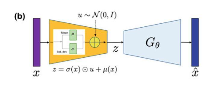
Each coordinate of \sigma_\phi(x) is positive, so Figure 4.1 realizes
q_\phi(z\mid x)=\mathcal N\!\left(\mu_\phi(x),\operatorname{diag}\big(\sigma_\phi^2(x)\big)\right),
and the Jacobian the general loss asks for is immediate:
\frac{\partial F_\phi^x(u)}{\partial u}=\operatorname{diag}\big(\sigma_\phi(x)\big), \qquad \log\left|\det\!\left(\frac{\partial F_\phi^x(u)}{\partial u}\right)\right| =\frac12\sum_{i=1}^d\log\sigma_i^2(x).
Note what is not required: the map from observations to codes need not be invertible. Only the map from noise to code, at fixed x, must be. This is the VAE of Kingma and Welling (Kingma and Welling 2014), and writing the sample this way is also what lets gradients reach \phi — see Section 4.12.2.
4.5.2 The Gaussian KL term
Let r and p both be standard Gaussian. Their normalizing constants cancel in the ratio, so
\log\!\left(\frac{r(u)}{p(F_\phi^x(u))}\right) =\tfrac12\left(\|\mu_\phi(x)+\sigma_\phi(x)\odot u\|^2-\|u\|^2\right),
and since \mathbb E[u_i]=0, \mathbb E[u_i^2]=1, the middle term of Equation 4.6 averages to \tfrac12\sum_i(\mu_i^2(x)+\sigma_i^2(x)-1). Adding the log-determinant gives the book’s (13.64)–(13.65):
D_{\mathrm{KL}}\!\left(q_\phi(z\mid x)\,\|\,\mathcal N(0,I_d)\right) =\frac12\sum_{i=1}^d\left(\sigma_i^2(x)+\mu_i^2(x)-\log\sigma_i^2(x)-1\right). \tag{4.8}
The variance part, \sigma_i^2-\log\sigma_i^2-1, is minimized at \sigma_i^2=1 and grows without bound in both directions, so the term penalizes a collapsed code and an over-dispersed one alike.
4.5.3 From likelihood to reconstruction error
With p_\theta(x\mid z)=\mathcal N(G_\theta(z),I_D),
-\log p_\theta(x\mid z)=\tfrac12\|x-G_\theta(z)\|^2+\tfrac D2\log(2\pi).
Two things are being used here and both matter: the observation model is Gaussian, and its covariance is the identity. Neither is forced on us — a Bernoulli decoder on binarized images gives a cross-entropy instead, and the squared-error form would then be wrong. Dropping the parameter-free constant and combining with Equation 4.8 gives the objective, the book’s (13.67):
\boxed{ \begin{aligned} \ell_{\mathrm{VAE}}(\theta,\phi) ={}&\frac12\int_{\mathcal X}\!\!\int \left\|x-G_\theta\!\left(\mu_\phi(x)+\sigma_\phi(x)\odot u\right)\right\|^2 r(u)\,du\,d\mu(x)\\ &+\frac12\sum_{i=1}^d\int_{\mathcal X} \left(\sigma_i^2(x)+\mu_i^2(x)-\log\sigma_i^2(x)-1\right)d\mu(x). \end{aligned}} \tag{4.9}
4.5.4 Varying the decoder output
After training, resampling the noise at a fixed observation traces out a family of reconstructions, the book’s (13.68):
\hat x(u)=G_\theta\!\left(\mu_\phi(x)+\sigma_\phi(x)\odot u\right), \qquad u\sim\mathcal N(0,I_d).
The encoder’s mean and spread stay fixed while u moves the code. This is the concrete sense in which a VAE is generative where a deterministic autoencoder is not; to generate without any input, draw z\sim p(z) instead.
4.6 The beta-VAE
Weighting the two terms differently gives the beta-VAE (Higgins et al. 2017), the book’s (13.69):
\boxed{ \begin{aligned} \ell_{\beta\text{-}\mathrm{VAE}}(\theta,\phi) ={}&\frac12\int_{\mathcal X}\!\!\int \left\|x-G_\theta\!\left(\mu_\phi(x)+\sigma_\phi(x)\odot u\right)\right\|^2 r(u)\,du\,d\mu(x)\\ &+\frac\beta2\sum_{i=1}^d\int_{\mathcal X} \left(\sigma_i^2(x)+\mu_i^2(x)-\log\sigma_i^2(x)-1\right)d\mu(x). \end{aligned}} \tag{4.10}
Setting \beta=1 recovers Equation 4.9. A larger \beta buys prior conformity with reconstruction detail. Section 4.12.4 derives \beta as a Lagrange multiplier on an information budget, which is where the choice stops looking arbitrary.
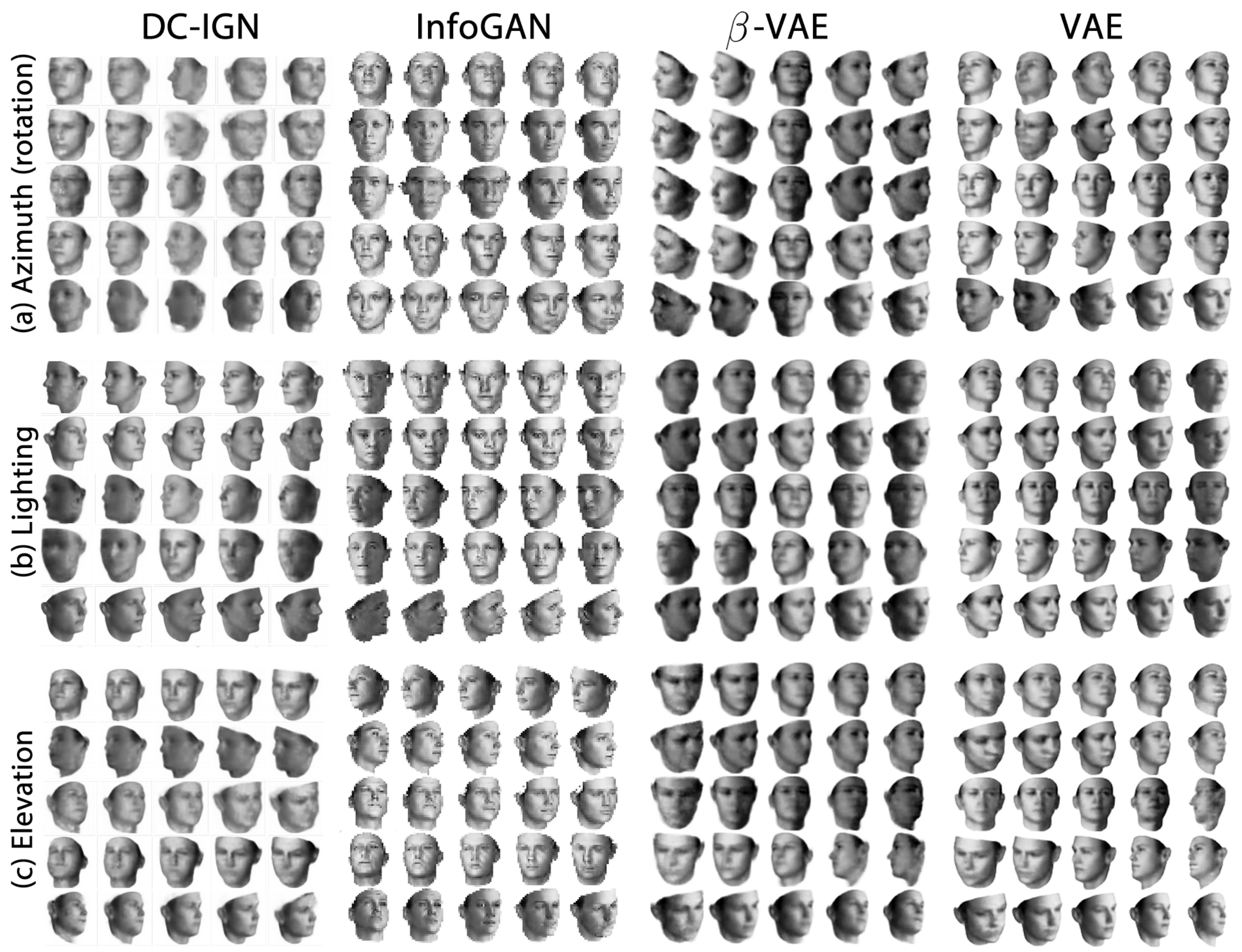
Figure 4.2 shows both halves of the trade at once. A coordinate is better aligned with a factor of variation when moving it moves that factor and little else, and the beta-VAE rows do this more consistently. They are also blurrier: under a squared-error objective a decoder that cannot distinguish fine detail averages it away. Stronger regularization can encourage interpretable structure; it does not guarantee it, and past some point it simply discards information.
4.7 Normalizing and invertible flows
4.7.1 Noise before an invertible map
Now make the encoder invertible and tie the decoder to it. Take D=d and F_\phi:\mathbb R^D\to\mathbb R^D invertible:
\boxed{ F_\phi^x(u)=F_\phi(\sigma u+x), \qquad G_\theta=F_\phi^{-1}, \qquad u\sim\mathcal N(0,I_D). } \tag{4.11}
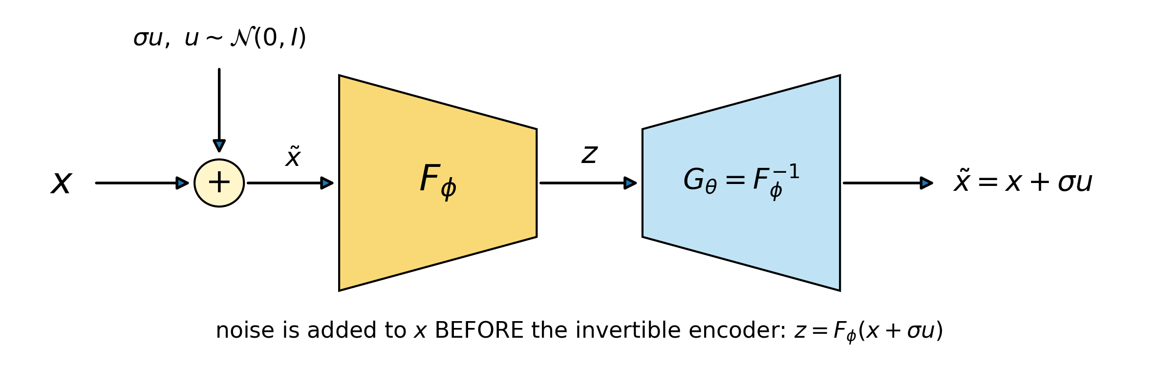
Here \sigma>0 is one fixed scalar, not the learned vector \sigma_\phi(x) of the VAE, and the encoder and decoder now share parameters. As Figure 4.3 records, the noise enters before the map; for a nonlinear F_\phi that is not the same as perturbing the output.
4.7.2 Why the reconstruction term becomes a constant
Because the decoder inverts the encoder exactly, reconstruction stops depending on the parameters at all:
\begin{aligned} \frac12\int\left\|x-G_\theta\!\left(F_\phi^x(u)\right)\right\|^2r(u)\,du &=\frac12\int\left\|x-F_\phi^{-1}\!\left(F_\phi(\sigma u+x)\right)\right\|^2r(u)\,du\\ &=\frac12\int\|\sigma u\|^2r(u)\,du=\frac{D\sigma^2}{2}. \end{aligned} \tag{4.12}
Since u\sim\mathcal N(0,I_D) we have \mathbb E\|u\|^2=D, so the value is D\sigma^2/2 — that is \sigma^2/2 per coordinate, which is how the slides write it (Ye 2026, 18). The conclusion is the same either way, because what matters is only that the term does not depend on \phi.
The entropy \int\log r\,r\,du is likewise parameter-free. Dropping both leaves the flow loss,
\begin{aligned} \ell_{\mathrm{flow}}(x,\phi) ={}&-\int\log p\!\left(F_\phi^x(u)\right)r(u)\,du\\ &-\int\log\left|\det\!\left(\frac{\partial F_\phi^x(u)}{\partial u}\right)\right|r(u)\,du , \end{aligned} \tag{4.13}
and with a standard Gaussian prior, up to one more constant,
\ell_{\mathrm{flow}}(x,\phi) =\frac12\int\|F_\phi(\sigma u+x)\|^2r(u)\,du -\int\log\left|\det\!\left(\frac{\partial F_\phi(\sigma u+x)}{\partial u}\right)\right|r(u)\,du .
Two forces are now in balance and neither alone would do. The prior term pulls latent outputs into the high-density region; left to itself it would collapse everything onto the origin. The log-determinant is what stops it: a map that crushes volume pays for it. Generation draws z\sim p(z) and applies G_\theta=F_\phi^{-1}.
4.7.3 Making the log-determinant tractable
A forward pass gives F_\phi(x) cheaply, but the determinant of a general network’s Jacobian does not come cheaply. Build F_\phi from simple invertible layers instead:
F_\phi=f_K\circ\cdots\circ f_1, \qquad h_0=x,\quad h_i=f_i(h_{i-1}),\quad h_K=F_\phi(x),
so that by the chain rule and multiplicativity of the determinant, the book’s (13.73)–(13.75),
\boxed{ \log\left|\det\!\left(\frac{\partial F_\phi(x)}{\partial x}\right)\right| =\sum_{i=1}^K\log\left|\det\!\left(\frac{\partial h_i}{\partial h_{i-1}}\right)\right| . } \tag{4.14}
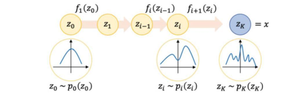
Composition turns a product into a sum, as Figure 4.4 illustrates, but it does not by itself make any single term cheap. Each layer still needs a Jacobian whose structure gives up its determinant, while the composition stays expressive enough to be worth having. For the noisy-input objective the layers start at h_0=\sigma u+x, and
\frac{\partial F_\phi(\sigma u+x)}{\partial u} =\left(\frac{\partial F_\phi(\sigma u+x)}{\partial x}\right)\sigma I_D ,
so the perturbation contributes a constant D\log\sigma and nothing else. Equation 4.13 is therefore the ordinary flow negative log density averaged over perturbed observations, up to parameter-free constants; Section 4.12.6 writes that density out and prices the dense determinant.
Generation reverses the order and inverts each layer, F_\phi^{-1}=f_1^{-1}\circ\cdots\circ f_K^{-1}, with f_K^{-1} acting first. The next two sections give layers for which both the inverse and the determinant are available in closed form.
4.8 NICE: additive coupling
4.8.1 The idea
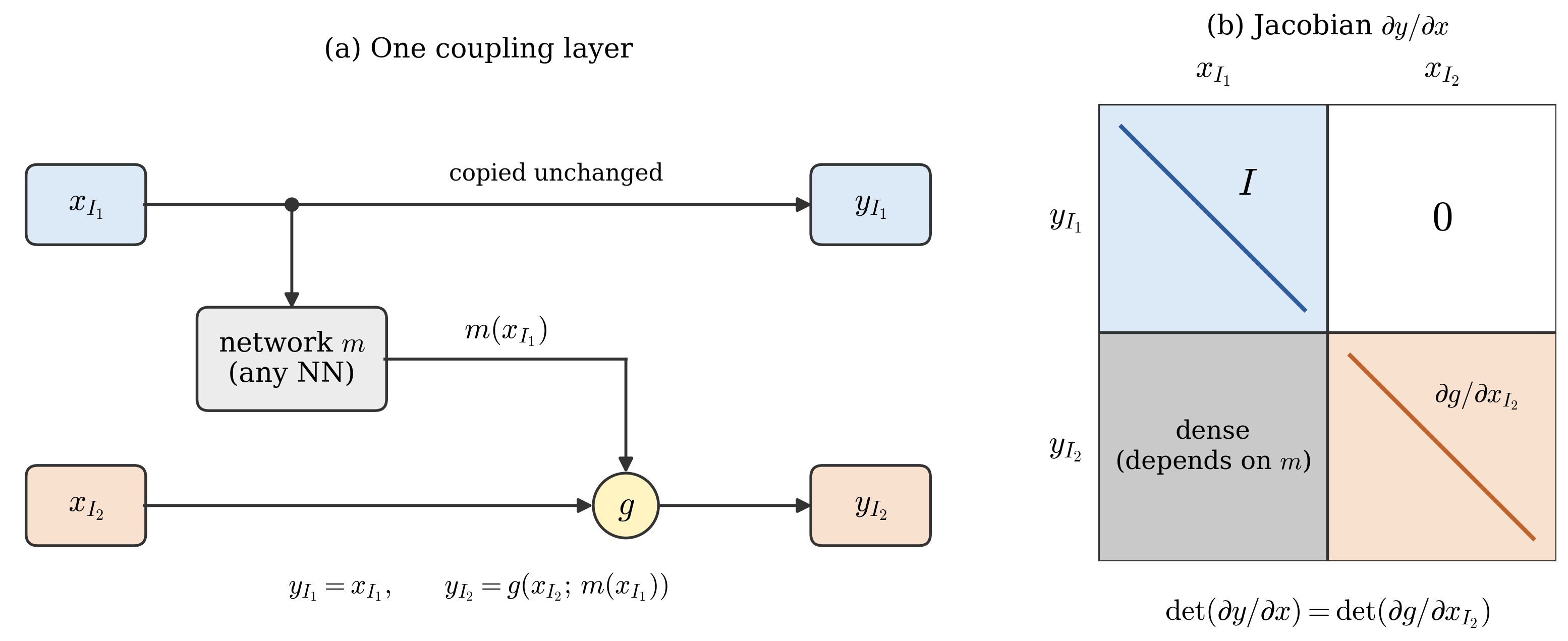
Figure 4.5 is the whole trick, and it is worth stating before any algebra. Split the coordinates. Copy one block. Let a network read the copied block and transform the other block with it. Because the copied block is available unchanged on both sides, the network’s output can be recomputed during inversion rather than inverted — so the network may be arbitrarily complicated while the layer stays exactly invertible.
4.8.2 Forward map, inverse, and Jacobian
Split x into x_1\in\mathbb R^m and x_2\in\mathbb R^{D-m} with 1\le m<D. NICE adds a network output to the second block (Dinh et al. 2015):
\boxed{ y_1=x_1,\qquad y_2=x_2+\mathcal F(x_1). } \tag{4.15}
The inverse recovers x_1 immediately and subtracts the same quantity,
\boxed{ x_1=y_1,\qquad x_2=y_2-\mathcal F(y_1), } \tag{4.16}
and the Jacobian is block triangular with identity diagonal blocks:
\frac{\partial y}{\partial x} =\begin{bmatrix} I_m & 0\\[2pt] \dfrac{\partial\mathcal F(x_1)}{\partial x_1} & I_{D-m}\end{bmatrix}, \qquad \log\left|\det\!\left(\frac{\partial y}{\partial x}\right)\right|=0 . \tag{4.17}
4.8.3 The loss, and the price of volume preservation
A composition of additive couplings and permutations has |\det(\partial F_\phi/\partial x)|=1, so every log-determinant in Equation 4.13 vanishes and, dropping constants,
\boxed{ \ell_{\mathrm{NICE}}(x,\phi)=\frac12\int\|F_\phi(\sigma u+x)\|^2 r(u)\,du . } \tag{4.18}
Training simply drives perturbed observations into the prior’s high-density region. The restriction is severe and easy to miss: additive layers can bend and reorient a region but can never change its volume, and stacking them does not help, since a product of ones is one. A flow built only from these layers cannot adapt the density of the prior to the density of the data, however complex the networks \mathcal F are. The original NICE model therefore ends with a learned diagonal scaling layer, which supplies the missing volume change and its own log-determinant (Dinh et al. 2015). Real NVP puts the scaling inside every layer instead.
4.9 Real NVP: affine coupling
4.9.1 Forward map and inverse
Real NVP gives the coupling an input-dependent scale (Dinh et al. 2017):
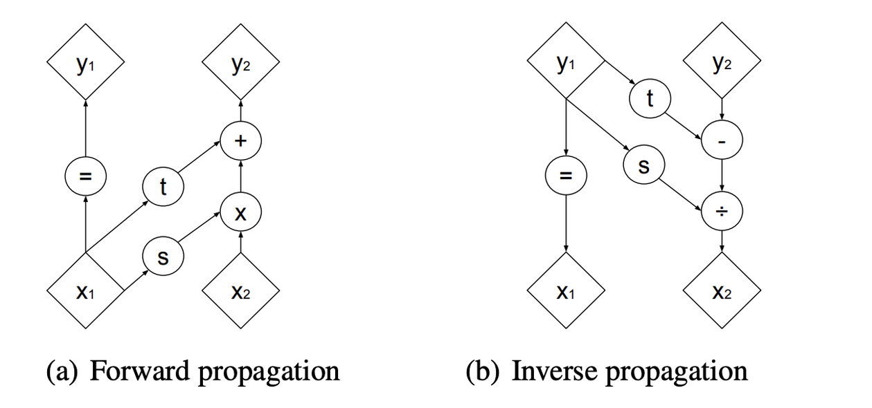
\boxed{ y_1=x_1,\qquad y_2=x_2\odot\exp\!\left(s(x_1)\right)+t(x_1), } \tag{4.19}
with s,t:\mathbb R^m\to\mathbb R^{D-m} producing log scales and translations. The exponential makes every scale positive, and s=0 recovers NICE. Inversion evaluates the same two networks at y_1=x_1:
\boxed{ x_1=y_1,\qquad x_2=\left(y_2-t(y_1)\right)\odot\exp\!\left(-s(y_1)\right). } \tag{4.20}
4.9.2 The determinant
Differentiating Equation 4.19, the lower-left block is whatever it is and the diagonal is what counts:
\frac{\partial y}{\partial x} =\begin{bmatrix} I_m & 0\\[2pt] \dfrac{\partial y_2}{\partial x_1} & \operatorname{diag}\!\left(\exp\!\left(s(x_1)\right)\right)\end{bmatrix}, \qquad \log\left|\det\!\left(\frac{\partial y}{\partial x}\right)\right| =\sum_j s_j(x_1). \tag{4.21}
A positive sum means the layer expands volume locally and a negative sum means it contracts. Section 4.12.8 carries a single layer through with numbers and checks this against a finite-difference Jacobian.
4.9.3 The loss
Let F_\phi=f_K\circ\cdots\circ f_1 be affine couplings with permutations between them, and write h_0(u)=\sigma u+x, h_i(u)=f_i(h_{i-1}(u)). Let s_{i,j} be the jth log-scale output of layer i, evaluated on that layer’s conditioning block h_{i-1,1}(u). Permutations contribute nothing, so combining Equation 4.21 with Equation 4.14 and dropping constants,
\boxed{ \ell_{\mathrm{RealNVP}}(x,\phi) =\int\left[\frac12\|F_\phi(\sigma u+x)\|^2 -\sum_{i=1}^K\sum_j s_{i,j}\!\left(h_{i-1,1}(u)\right)\right]r(u)\,du . } \tag{4.22}
Setting every log-scale network to zero returns Equation 4.18. The translation networks never appear in the determinant, yet they shape the loss through the states h_i. For ordinary density estimation, run the same layers at h_0=x:
-\log p_X(x)=\frac12\|F_\phi(x)\|^2-\sum_{i=1}^K\sum_j s_{i,j}(h_{i-1,1})+\frac D2\log(2\pi). \tag{4.23}
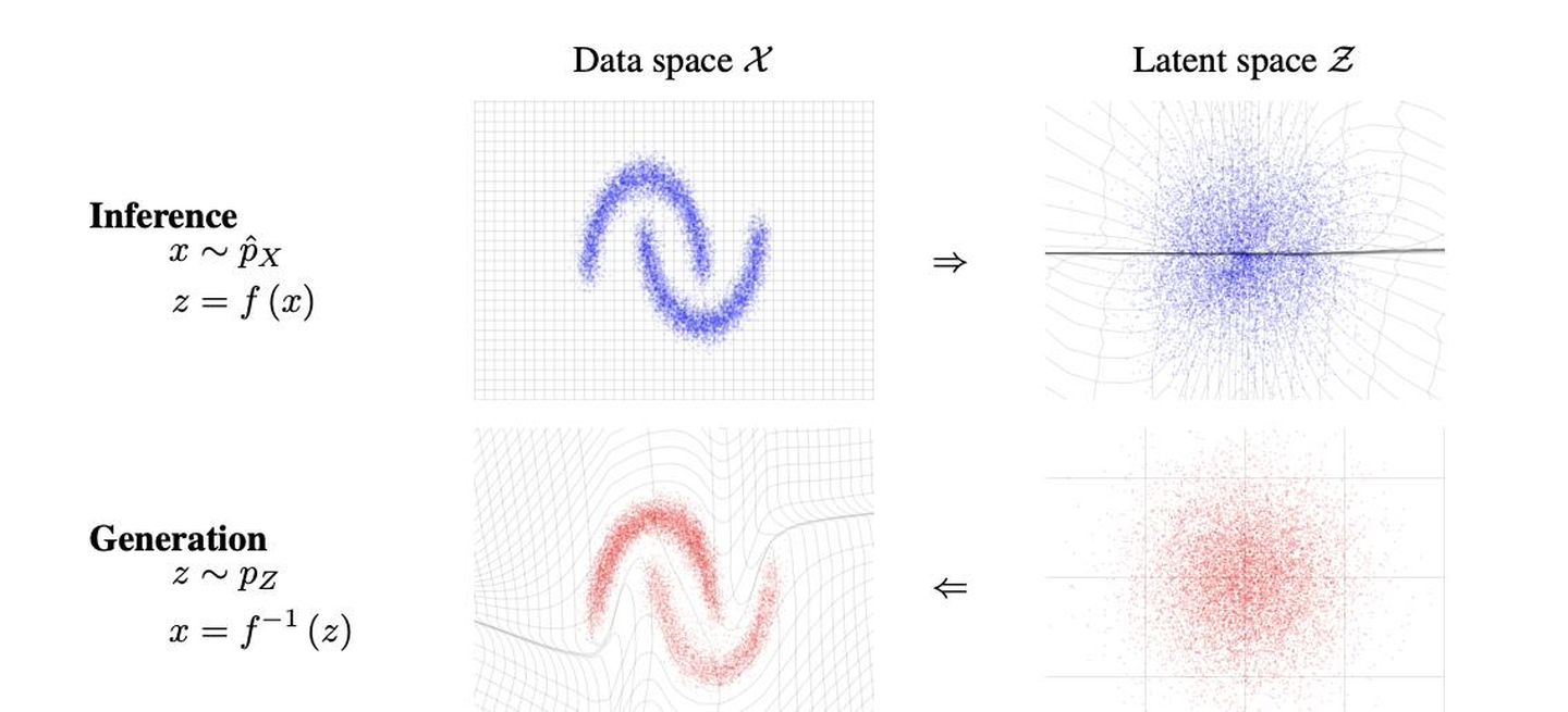
Figure 4.7 makes the point that a trained flow is one bijection: inference and generation are not two models but two ways of reading the same one.
4.10 Glow
The lecture closes with Glow (Kingma and Dhariwal 2018), which keeps the coupling layer and fixes what coupling alone cannot do. A coupling layer always leaves one block untouched, so some coordinates must be permuted between layers for information to reach everything. A fixed permutation is a crude instrument. Glow replaces it with a learned one and adds a normalization layer, giving three components per step (Ye 2026, 23–25, 36–41).
Actnorm. A per-channel affine transform y_{i,j}=s\odot x_{i,j}+b applied at every spatial position (i,j) of an h\times w\times c tensor, initialized so that the post-transform activations have zero mean and unit variance on the first minibatch. Its log-determinant is h\cdot w\cdot\operatorname{sum}(\log|s|).
Invertible 1\times1 convolution. The learned replacement for a fixed permutation: y_{i,j}=Wx_{i,j} with W a c\times c matrix shared across positions. Because the same matrix acts at every one of the h\cdot w positions,
\log\left|\det\!\left(\frac{\partial\,\mathrm{conv2D}(h;W)}{\partial h}\right)\right| =h\cdot w\cdot\log\left|\det W\right| . \tag{4.24}
A permutation matrix is a special case, so the layer can only improve on one. Computing \det W directly costs O(c^3); parameterizing W in LU form removes that:
W=PL\left(U+\operatorname{diag}(s)\right), \qquad \log|\det W|=\operatorname{sum}\left(\log|s|\right), \tag{4.25}
with P a fixed permutation, L unit lower triangular and U strictly upper triangular, bringing the cost to O(c).
Affine coupling. Exactly Equation 4.19, acting on a channel split, with log-determinant \operatorname{sum}(\log|s|).
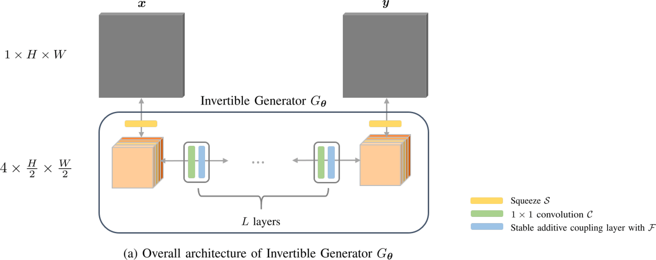
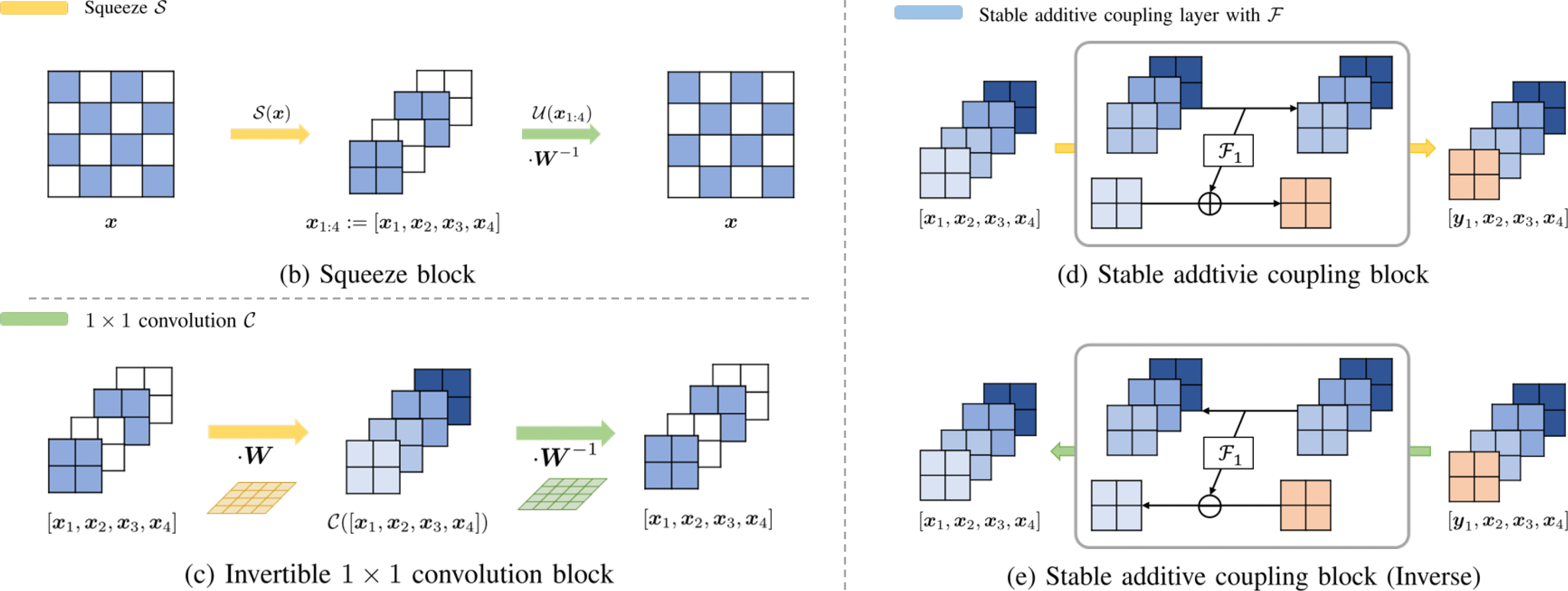
Figure 4.8 and Figure 4.9 are worth reading together: the first says the model is a stack, the second says every element of the stack is a map whose inverse is written next to it. That is the whole design constraint of this chapter made concrete.
A squeeze operation between scales trades spatial resolution for channels, reshaping 1\times H\times W into 4\times\frac H2\times\frac W2, so that the 1\times1 convolution has channels to mix and the coupling split is spatially local. Stacking L such steps gives the invertible generator; every component has a closed-form inverse and an O(c) log-determinant, so Equation 4.14 applies unchanged and the model is trained by exact maximum likelihood.
The point is not the particular three layers. It is that the whole chapter’s constraint — invertible, with a cheap determinant — has enough room inside it to build a model that samples high-resolution images, provided each layer’s structure is chosen so that its determinant is read off rather than computed.
4.11 What the coupling construction costs
Flows must be expressive, invertible, and cheap to differentiate, and the three demands pull against each other. Setting y_1=x_1 buys the triangular Jacobian, and the price is that no single layer can transform all coordinates jointly: each one leaves a block alone and moves the rest by a restricted affine map. Alternating the blocks lets every coordinate change eventually, but a restricted layer may need a deep stack to express what one unrestricted map would, and depth is compute. NICE pays more than Real NVP, being confined to unit volume.
Two limits are structural rather than architectural. A bijection forces D=d, so a flow has no bottleneck and no compressed representation — exactly what the VAE gives up invertibility to obtain. And scale factors that grow very large or very small make numerical inversion ill-conditioned, which bounds in practice how aggressive the learned volume changes can be.
4.12 Advanced topics
The material below was not developed in the lecture. It is collected here so that the preceding sections follow the class.
4.12.1 The ELBO gap, exactly
Write \mathcal L(x,\theta,\phi)=-\ell_{\mathrm{ELBO}}(x,\theta,\phi). Bayes’ rule gives a second derivation of the bound that also names the gap (Kingma and Welling 2014). Assuming finite expectations,
\begin{aligned} D_{\mathrm{KL}}\!\left(q_\phi(z\mid x)\,\|\,p_\theta(z\mid x)\right) &=\int q_\phi(z\mid x)\log\!\left(\frac{q_\phi(z\mid x)p_\theta(x)}{p_\theta(x,z)}\right)dz\\ &=\log p_\theta(x)-\mathcal L(x,\theta,\phi), \end{aligned}
so that
\log p_\theta(x)=\mathcal L(x,\theta,\phi) +D_{\mathrm{KL}}\!\left(q_\phi(z\mid x)\,\|\,p_\theta(z\mid x)\right). \tag{4.26}
The KL term is nonnegative, which proves the bound, and it is exactly the gap, vanishing when the encoder matches the true posterior almost everywhere. Note which two distributions it compares: the encoder and the posterior. The regularizer in Equation 4.3 compares the encoder with the prior. They are different objects and only the first is the bound’s slack.
4.12.2 Reparameterization and gradient estimation
Fix x and \theta and write f_\theta(z)=\log p_\theta(x\mid z). The reconstruction expectation depends on \phi through the distribution it averages over, which is not something a sampler can differentiate. Reparameterization moves that dependence into the integrand:
\mathbb E_{q_\phi(z\mid x)}\!\left[f_\theta(z)\right] =\mathbb E_{u\sim r}\!\left[f_\theta\!\left(F_\phi^x(u)\right)\right],
and since r does not depend on \phi, differentiating under the expectation gives the pathwise estimator
\nabla_\phi\mathbb E_q\!\left[f_\theta(z)\right] =\mathbb E_{u\sim r}\!\left[ \left(\frac{\partial F_\phi^x(u)}{\partial\phi}\right)^{\!\top} \left.\nabla_z f_\theta(z)\right|_{z=F_\phi^x(u)}\right]. \tag{4.27}
The alternative differentiates the density, using \nabla_\phi q=q\nabla_\phi\log q:
\nabla_\phi\int f_\theta(z)q_\phi(z\mid x)\,dz =\mathbb E_q\!\left[f_\theta(z)\nabla_\phi\log q_\phi(z\mid x)\right]. \tag{4.28}
This is the score-function estimator. Both are unbiased. The pathwise one uses \nabla_z f_\theta, first-order information about how the integrand moves when the code moves; the score-function one uses only the value f_\theta(z), weighted by a score. For a smooth Gaussian problem the first is usually far less noisy, and Section 4.12.3 makes the gap concrete — but this is a tendency, not a theorem. The score-function estimator remains the one that works when no differentiable reparameterization exists, as with discrete latent variables, and a baseline independent of z reduces its variance at no bias, since \mathbb E_q[\nabla_\phi\log q_\phi]=0.
4.12.3 Worked example: two gradient estimators
Take q_\mu=\mathcal N(\mu,1) and f(z)=z, so that \nabla_\mu\mathbb E_{q_\mu}[z]=1 for every \mu, and write z=\mu+u with u\sim\mathcal N(0,1).
The pathwise estimator Equation 4.27 gives \nabla_z f\cdot\partial z/\partial\mu=1 for every sample: exact, with zero variance. The score-function estimator Equation 4.28 uses \nabla_\mu\log q_\mu(z)=z-\mu=u, so one sample gives f(z)u=(\mu+u)u=\mu u+u^2, with mean 1 — also unbiased. For the variance, using \mathbb E[u^2]=1, \mathbb E[u^3]=0, \mathbb E[u^4]=3:
\operatorname{Var}(\mu u+u^2) =\mu^2\mathbb E[u^2]+2\mu\mathbb E[u^3]+\mathbb E[u^4]-1=\mu^2+2 . \tag{4.29}
| \mu | score function: mean | score function: variance | \mu^2+2 | pathwise: variance |
|---|---|---|---|---|
| 0 | 1.0013 | 2.007 | 2 | 0.0 |
| 1 | 0.9988 | 3.003 | 3 | 0.0 |
| 2 | 0.9965 | 5.980 | 6 | 0.0 |
| 3 | 0.9972 | 10.999 | 11 | 0.0 |
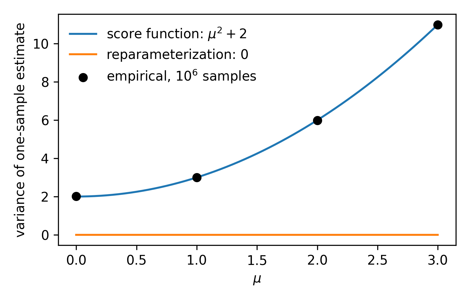
Table 4.1 and Figure 4.10 agree with Equation 4.29 to three figures. The variance grows with \mu^2, and in a VAE the role of f is played by \log p_\theta(x\mid z), a sum over thousands of pixels whose magnitude dwarfs \mu here. That is the practical reason the VAE is trained with Equation 4.27.
4.12.4 The beta-VAE as constrained rate-distortion
Define average distortion and rate by
\mathcal D(\theta,\phi)=-\int\mathbb E_{q_\phi(z\mid x)}\!\left[\log p_\theta(x\mid z)\right]d\mu(x), \qquad \mathcal R(\phi)=\int D_{\mathrm{KL}}\!\left(q_\phi(z\mid x)\,\|\,p(z)\right)d\mu(x).
Constraining the rate to a budget C and introducing a multiplier (Higgins et al. 2017),
\min_{\theta,\phi}\mathcal D \ \ \text{s.t.}\ \ \mathcal R\le C \qquad\Longrightarrow\qquad \mathcal J=\mathcal D+\beta\left(\mathcal R-C\right),\ \beta\ge0,
and since -\beta C is constant in the parameters, minimizing \mathcal J is minimizing \mathcal D+\beta\mathcal R — the beta-VAE objective (Burgess et al. 2018). Writing \mathcal D^*(\mathcal R) for the best distortion at a given rate, an interior smooth optimum satisfies \beta=-d\mathcal D^*/d\mathcal R, so \beta is the exchange rate between nats of latent information and reconstruction error. With nonconvex networks there is no guarantee that every budget C is attained by some fixed \beta.
The rate decomposes. With the aggregate encoder q_\phi(z)=\int q_\phi(z\mid x)\,d\mu(x), splitting the log ratio gives
\mathcal R=I_q(X,Z)+D_{\mathrm{KL}}\!\left(q_\phi(z)\,\|\,p(z)\right), \tag{4.30}
so the KL penalty is charging for two different things at once: the information the code keeps about the observation, and the mismatch between the aggregate code distribution and the prior.
4.12.5 Posterior collapse
Collapse is the state in which the latent variable carries nothing. At the extreme the decoder ignores z, so p_\theta(x\mid z)=p_\theta(x), hence p_\theta(z\mid x)=p(z); an encoder matching that posterior has q_\phi(z\mid x)=p(z) and, by Equation 4.30, zero rate and zero mutual information. Partial collapse switches off some coordinates and not others.
The failure is most likely exactly where it is least wanted: when the decoder is powerful enough to model the data on its own, the KL term is a pure cost and the cheapest way to pay it is to stop using the code. Large \beta encourages this, but it happens at \beta=1 too, and inference lag during joint training can drive a model there on its own (He et al. 2019). The symptoms under a standard Gaussian prior are \mu_\phi(x)\approx0, \sigma_\phi(x)\approx\mathbf 1 and a near-zero KL.
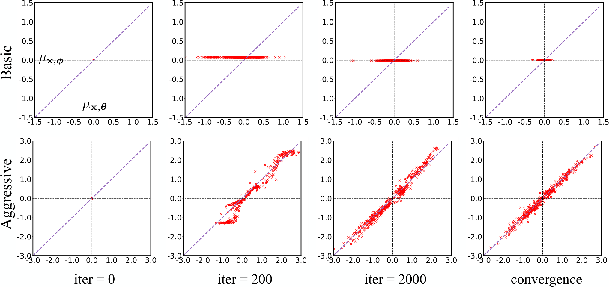
Figure 4.11 is a diagnosis, not a definition: spread along the diagonal says the encoder means still depend on the input. Means alone do not establish that two distributions agree, and blurry reconstructions on their own do not establish collapse. A common remedy is KL annealing, which starts training with a small weight on the KL term and raises it.
4.12.6 Exact flow densities and the cost of a determinant
For a differentiable bijection z=F_\phi(x) with nonsingular Jacobian, let p_X be the density induced by pushing the prior through F_\phi^{-1}; this is a model density, distinct from the data measure \mu. Conservation of probability, p_X(x)\,dx=p_Z(z)\,dz, gives
-\log p_X(x)=-\log p_Z\!\left(F_\phi(x)\right) -\log\left|\det\!\left(\frac{\partial F_\phi(x)}{\partial x}\right)\right| . \tag{4.31}
With a standard Gaussian prior the first term is \frac12\|F_\phi(x)\|^2 plus a constant, recovering Equation 4.23. The noisy-input objective of Section 4.7 averages this at x+\sigma u instead of at x.
The cost this chapter has been avoiding: a dense D\times D Jacobian needs O(D^2) storage and O(D^3) operations for an LU-based determinant, before counting the differentiation that builds it. Decomposition makes the log-determinants additive, but additivity alone saves nothing unless each term is cheap (Rezende and Mohamed 2015).
4.12.7 Planar and autoregressive layers
Coupling is one way to meet the requirement; two others are standard.
Planar flows. A rank-one perturbation of the identity (Rezende and Mohamed 2015),
f(x)=x+v\,h\!\left(w^\top x+b\right), \qquad v,w\in\mathbb R^D,\ b\in\mathbb R,
with h a differentiable scalar activation. The matrix determinant lemma \det(I+ab^\top)=1+b^\top a reduces the determinant to
\log\left|\det\!\left(\frac{\partial f(x)}{\partial x}\right)\right| =\log\left|1+h'\!\left(w^\top x+b\right)w^\top v\right| , \tag{4.32}
an O(D) computation. Invertibility is not automatic and the condition is easy to omit: for h=\tanh it requires w^\top v>-1, without which the determinant can vanish or change sign and Equation 4.31 no longer applies. Under that condition, with a=w^\top x+b, the scalar map a\mapsto a+(w^\top v)\tanh a has positive derivative and is onto, so a and then x=y-v\tanh a are determined — but only through a numerical solve, unlike the closed-form inverse of a coupling layer. Planar layers are therefore used to enrich a variational posterior rather than to model data.
Autoregressive flows. Here x_i and y_i are scalar coordinates, not the vector blocks of the coupling sections. With x_{<i}=(x_1,\ldots,x_{i-1}),
y_i=x_i\exp\!\left(s_i(x_{<i})\right)+t_i(x_{<i}), \qquad i=1,\ldots,D,
the Jacobian is triangular and \log|\det\partial f/\partial x|=\sum_i s_i(x_{<i}). Masked networks compute every s_i,t_i in one parallel pass when the full input is known, while the other direction is sequential because x_{<i} must be recovered first. MAF takes the parallel direction for density evaluation; IAF takes it for sampling (Papamakarios et al. 2017; Kingma et al. 2016). A coupling layer is the two-block special case: less expressive per layer, fast in both directions.
Planar layers exploit a rank-one update, coupling layers a block-triangular split, autoregressive layers a coordinate ordering, and Glow a matrix factorization. In every case the determinant is made cheap by structure, not by computation.
4.12.8 Worked example: one affine coupling layer by hand
Two dimensions, D=2 with split index m=1. Let the flow be a single affine coupling with s(x_1)=\tfrac12 x_1 and t(x_1)=-x_1^2, so
z_1=x_1,\qquad z_2=x_2\exp\!\left(\tfrac12 x_1\right)-x_1^2, \qquad z\sim\mathcal N(0,I_2). \tag{4.33}
Forward. At x=(1,0.5): s=0.5, t=-1, so z_1=1 and z_2=0.5e^{0.5}-1=-0.17564.
Log-determinant. By Equation 4.21 it is just s(x_1)=0.5. Writing the full Jacobian shows what drops out:
\frac{\partial z}{\partial x} =\begin{bmatrix}1&0\\ \tfrac12 x_2e^{x_1/2}-2x_1 & e^{x_1/2}\end{bmatrix} =\begin{bmatrix}1&0\\ -1.58782 & 1.64872\end{bmatrix}, \qquad\det=e^{0.5}=1.64872 .
The lower-left entry involves both s and t; the determinant never sees it.
Log-likelihood. By Equation 4.31 with p_Z=\mathcal N(0,I_2),
\log p_X(x)=-\log 2\pi-\tfrac12\|z\|^2+s(x_1) =-1.83788-\tfrac12(1+0.03085)+0.5=-1.85330 .
Inverse. x_2=(z_2-t(z_1))e^{-s(z_1)}=(-0.17564+1)e^{-0.5}=0.5, recovering x exactly, with s and t evaluated and never inverted.
| Quantity | By hand | Numerical check |
|---|---|---|
| z=F(x) | (1,-0.17564) | (1,-0.17564) |
| \log\lvert\det\partial z/\partial x\rvert | s(x_1)=0.5 | \log 1.64872=0.5 (finite differences) |
| \log p_X(x) | -1.85330 | -1.85330 |
| F^{-1}(F(x)) | (1,0.5) | (1,0.5) |
| \int p_X\,dx | 1 | 0.9999999981 |
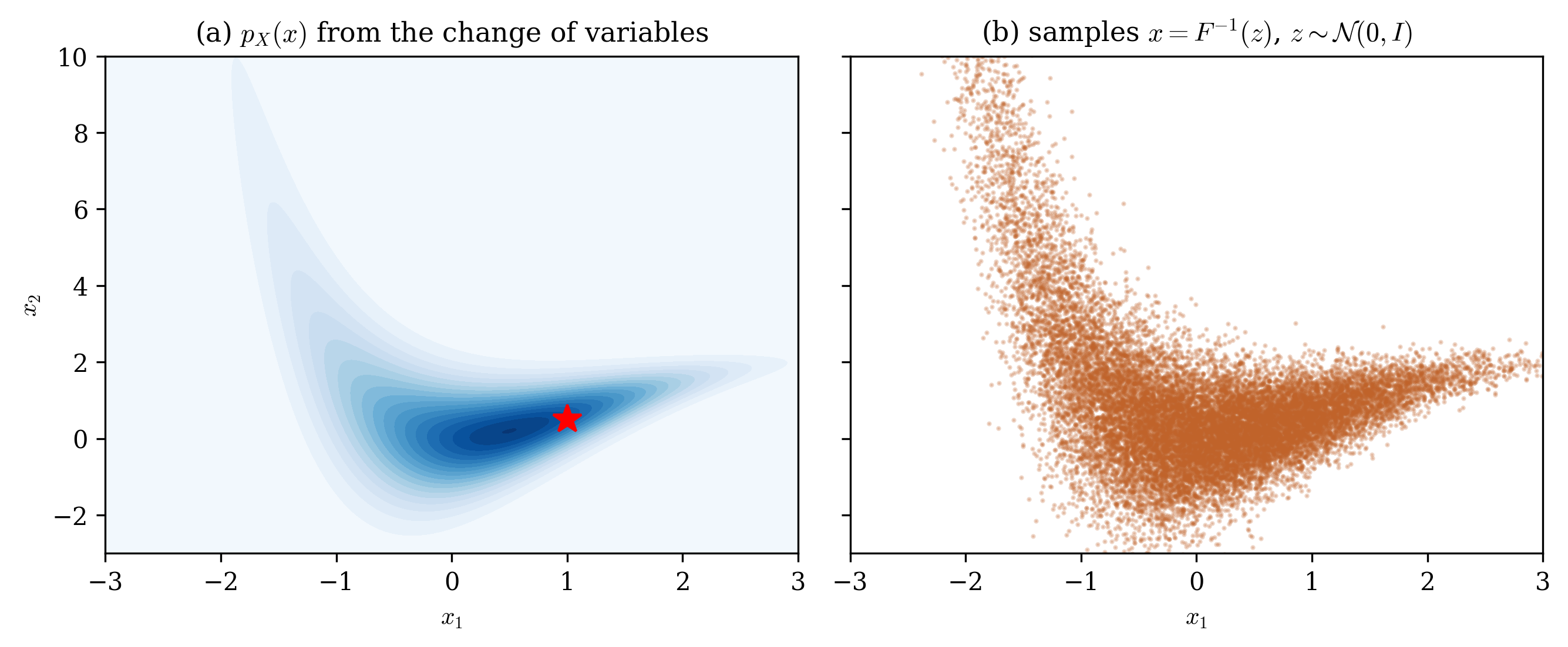
The normalization in Table 4.2 is computed one x_1 at a time, since \int p_X(x_1,x_2)\,dx_2=\mathcal N(x_1;0,1) for every x_1. Figure 4.12 shows what one layer does: z_2 is shifted by -x_1^2 and rescaled by e^{x_1/2}, so the Gaussian bends into a curved ridge. One layer can only bend x_2 as a function of x_1. Alternating the roles of the two coordinates across layers is what lets a flow bend in both directions.
4.12.9 Where this chapter leads
| Model | Encoder F_\phi^x | \dim z | Objective | \log\lvert\det\rvert cost | Inverse |
|---|---|---|---|---|---|
| VAE (Kingma and Welling 2014) | Gaussian, Equation 4.7 | d<D | ELBO | closed form | not needed |
| beta-VAE (Higgins et al. 2017) | same | d<D | \mathcal D+\beta\mathcal R | closed form | not needed |
| NICE (Dinh et al. 2015) | additive coupling | D | exact likelihood | 0 | one pass |
| Real NVP (Dinh et al. 2017) | affine coupling | D | exact likelihood | O(D) | one pass |
| Glow (Kingma and Dhariwal 2018) | coupling + 1\times1 conv | D | exact likelihood | O(c) per conv | one pass |
| Planar (Rezende and Mohamed 2015) | Equation 4.32 | D | posterior only | O(D) | numerical solve |
| MAF / IAF (Papamakarios et al. 2017; Kingma et al. 2016) | autoregressive | D | exact likelihood | O(D) | sequential one way |
Read Table 4.3 down the \dim z column and the chapter’s one trade-off is visible: the VAE compresses and pays with an approximate likelihood; every flow keeps the likelihood exact and pays by giving up the bottleneck.
Diffusion models, the subject of the next part, take the flow’s picture of generation as a chain of invertible steps and push it to the continuous limit. The chain becomes a stochastic differential equation, the sum of log-determinants becomes an integral, and the network defining the dynamics no longer needs the explicitly invertible coupling architecture that NICE, Real NVP and Glow were built around (Song et al. 2021).
Based on the scribe note of Jungwoo Park, with material from Youngjin Shin and Daehan Yoon; edited by Jong Chul Ye.